Code
library(tidyverse)
theme_set(theme_minimal(base_size = 11))
Due Wednesday, November 18, 2026, 11:59 pm (Pacific)
This study guide will help you prepare for the STAT 204 exam covering:
Exam Format:
|>AI and studying: AI use is encouraged for studying (see the syllabus AI Policy), but solve each problem yourself first. Where AI would fail here: it can give confident but incorrect worked solutions, misread an interpretation, or explain a diagnostic plot it cannot see. Check every AI answer against the class notes. The exam is closed-book with no AI, so practice without it. Do not upload course materials (including this guide) to AI platforms.
All datasets below come from TidyTuesday and are read directly from GitHub, so you can run every chunk yourself.
library(tidyverse)
theme_set(theme_minimal(base_size = 11))set.seed() before anything random)lm) output: which coefficients to addThese are the kinds of formulas worth putting on your formula sheet. Your sheet must contain formulas only.
The first two problems use Spotify songs (TidyTuesday, January 21, 2020): audio features for songs from playlists of six genres. danceability and energy run from 0 to 1, loudness is in decibels (0 dB is the loudest), and mode is major or minor. Songs that appeared in several playlists were listed more than once in the raw file.
spotify_raw <- read_csv("https://raw.githubusercontent.com/rfordatascience/tidytuesday/master/data/2020/2020-01-21/spotify_songs.csv")
nrow(spotify_raw)
[1] 32833# JUDGMENT CALL: keep one row per song (track_id); the raw file lists
# a song once for every playlist it appears in.
spotify <- spotify_raw |>
distinct(track_id, .keep_all = TRUE) |>
mutate(playlist_genre = factor(playlist_genre),
mode = factor(mode, levels = 0:1, labels = c("minor", "major")))
nrow(spotify)[1] 28356ggplot(spotify, aes(x = playlist_genre, y = danceability)) +
geom_boxplot(fill = "grey85", outlier.alpha = 0.4) +
labs(x = "Playlist genre", y = "Danceability")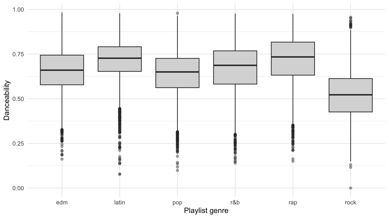
An analyst reports: “Rap and latin are the most danceable genres, and rock is the least.” They checked it like this:
set.seed(204)
spotify <- spotify |>
  mutate(half = sample(rep(c("explore", "hold out"), length.out = n())))

# median danceability by genre in each half
spotify |>
  group_by(playlist_genre, half) |>
  summarise(median = round(median(danceability), 3), .groups = "drop") |>
  pivot_wider(names_from = half, values_from = median)
# A tibble: 6 × 3
playlist_genre explore `hold out`
<fct> <dbl> <dbl>
1 edm 0.659 0.661
2 latin 0.725 0.728
3 pop 0.647 0.652
4 r&b 0.685 0.689
5 rap 0.734 0.734
6 rock 0.518 0.524Questions:
set.seed(204)
# JUDGMENT CALL: plot a random 3,000 songs so the points are readable
sub <- slice_sample(spotify, n = 3000)

ggplot(sub, aes(x = loudness, y = energy, color = mode)) +
  geom_point(alpha = 0.5, size = 1) +
  scale_color_manual(values = c("minor" = "#0072B2", "major" = "#D55E00")) +
  labs(x = "Loudness (dB)", y = "Energy", color = "Mode") +
  theme(legend.position = "top")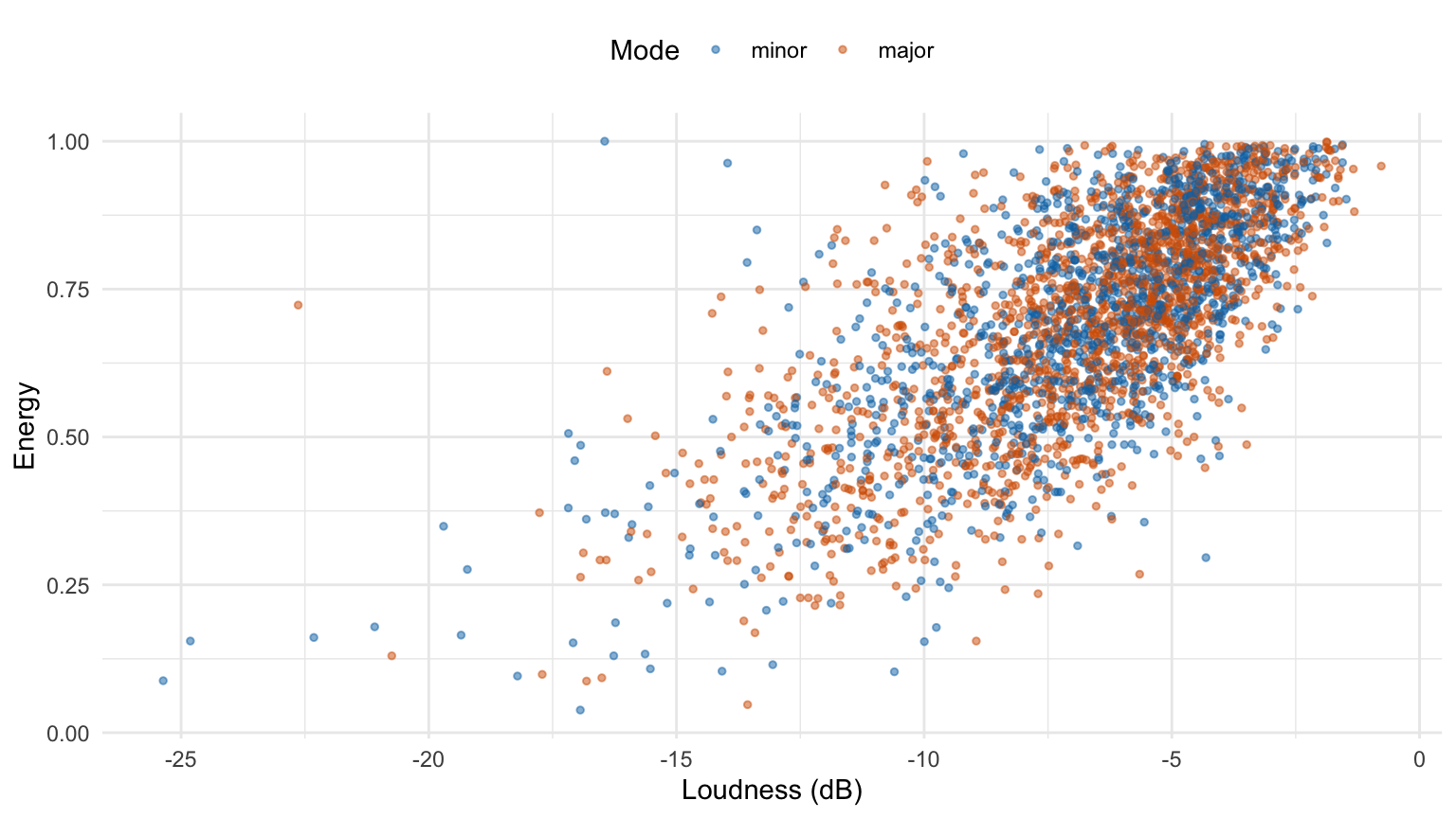
Questions:
Chocolate bar ratings (TidyTuesday, January 18, 2022): expert ratings (1 to 4, in steps of 0.25) of 2,530 dark chocolate bars, along with their cocoa percentage.
chocolate <- read_csv("https://raw.githubusercontent.com/rfordatascience/tidytuesday/master/data/2022/2022-01-18/chocolate.csv") |>
  mutate(cocoa = parse_number(cocoa_percent))

M1 <- lm(rating ~ cocoa, data = chocolate)
summary(M1)
Call:
lm(formula = rating ~ cocoa, data = chocolate)

Residuals:
     Min       1Q   Median       3Q      Max
-2.21541 -0.23867  0.03459  0.28459  0.99393

Coefficients:
            Estimate Std. Error t value Pr(>|t|)
(Intercept)  4.02953    0.11209  35.949  < 2e-16 ***
cocoa       -0.01163    0.00156  -7.456 1.22e-13 ***
---
Signif. codes:  0 '***' 0.001 '**' 0.01 '*' 0.05 '.' 0.1 ' ' 1

Residual standard error: 0.4406 on 2528 degrees of freedom
Multiple R-squared:  0.02152,   Adjusted R-squared:  0.02113
F-statistic: 55.59 on 1 and 2528 DF,  p-value: 1.218e-13
Questions:
par(mfrow = c(1, 2))
plot(M1, which = 1, main = "Residuals vs Fitted", caption = "")
plot(M1, which = 2, main = "Q-Q Residuals", caption = "")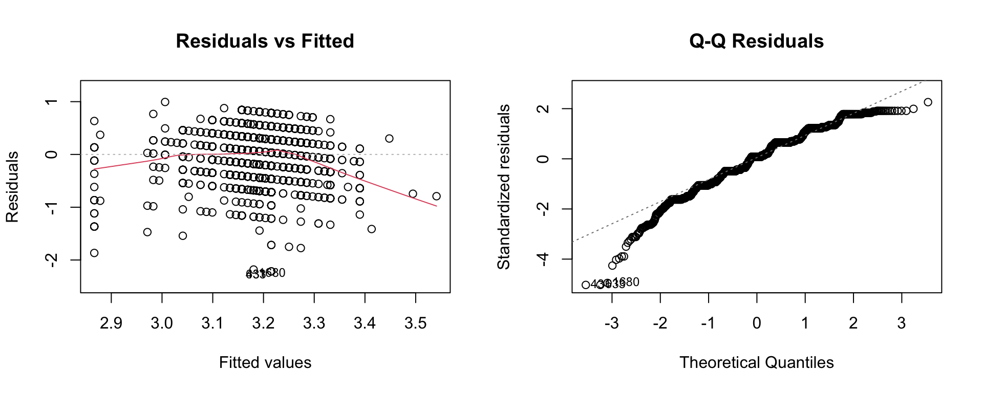
par(mfrow = c(1, 1))Questions:
rating take?) Is this a violation?Using the Spotify data, an analyst keeps three genres and fits a two-way ANOVA with interaction:
songs <- spotify |>
  filter(playlist_genre %in% c("pop", "rap", "rock")) |>
  mutate(playlist_genre = droplevels(playlist_genre))

table(songs$playlist_genre, songs$mode)
       minor major
  pop   2094  3038
  rap   2578  2823
rock 1323 2982M2 <- lm(danceability ~ playlist_genre * mode, data = songs)
summary(M2)
Call:
lm(formula = danceability ~ playlist_genre * mode, data = songs)

Residuals:
     Min       1Q   Median       3Q      Max
-0.56901 -0.08499  0.01201  0.09499  0.43476

Coefficients:
                              Estimate Std. Error t value Pr(>|t|)
(Intercept)                   0.648886   0.002948 220.129  < 2e-16 ***
playlist_genrerap             0.063798   0.003968  16.077  < 2e-16 ***
playlist_genrerock           -0.136508   0.004737 -28.815  < 2e-16 ***
modemajor                    -0.018899   0.003831  -4.933 8.19e-07 ***
playlist_genrerap:modemajor   0.025226   0.005309   4.752 2.03e-06 ***
playlist_genrerock:modemajor  0.027765   0.005876   4.725 2.33e-06 ***
---
Signif. codes:  0 '***' 0.001 '**' 0.01 '*' 0.05 '.' 0.1 ' ' 1

Residual standard error: 0.1349 on 14832 degrees of freedom
Multiple R-squared:  0.2589,    Adjusted R-squared:  0.2586
F-statistic:  1036 on 5 and 14832 DF,  p-value: < 2.2e-16
Questions:
modemajor coefficient. Which genre does it apply to?anova(M2)Analysis of Variance Table
Response: danceability
Df Sum Sq Mean Sq F value Pr(>F)
playlist_genre 2 93.705 46.853 2574.9999 < 2.2e-16 ***
mode 1 0.013 0.013 0.7206 0.396
playlist_genre:mode 2 0.556 0.278 15.2681 2.377e-07 ***
Residuals 14832 269.872 0.018
---
Signif. codes: 0 '***' 0.001 '**' 0.01 '*' 0.05 '.' 0.1 ' ' 1songs |>
group_by(playlist_genre, mode) |>
summarise(mean_dance = mean(danceability), .groups = "drop") |>
ggplot(aes(x = mode, y = mean_dance, color = playlist_genre, group = playlist_genre)) +
geom_line(linewidth = 1.1) +
geom_point(size = 3) +
scale_color_manual(values = c("#0072B2", "#D55E00", "#009E73")) +
labs(x = "Mode", y = "Mean danceability", color = "Genre")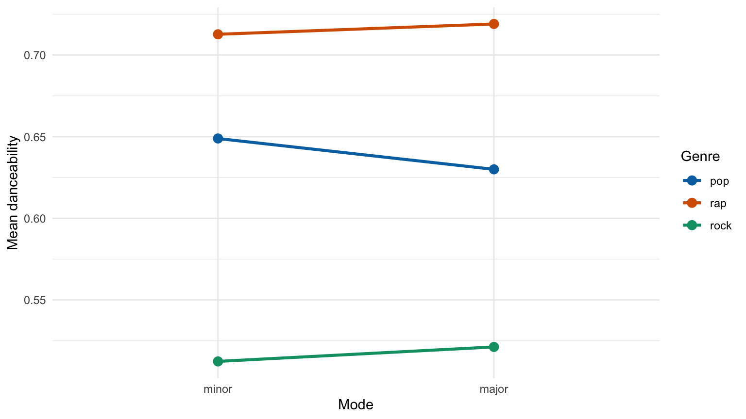
Questions:
M3 <- lm(energy ~ loudness, data = spotify)
summary(M3)
Call:
lm(formula = energy ~ loudness, data = spotify)

Residuals:
     Min       1Q   Median       3Q      Max
-0.54304 -0.08864  0.00586  0.09173  1.36044

Coefficients:
             Estimate Std. Error t value Pr(>|t|)
(Intercept) 0.9794588  0.0019587   500.0   <2e-16 ***
loudness    0.0412267  0.0002625   157.1   <2e-16 ***
---
Signif. codes:  0 '***' 0.001 '**' 0.01 '*' 0.05 '.' 0.1 ' ' 1

Residual standard error: 0.1342 on 28354 degrees of freedom
Multiple R-squared:  0.4653,    Adjusted R-squared:  0.4653
F-statistic: 2.468e+04 on 1 and 28354 DF, p-value: < 2.2e-16ggplot(sub, aes(x = loudness, y = energy)) +
geom_point(alpha = 0.3, size = 0.8, color = "grey40") +
geom_smooth(method = "lm", se = FALSE, color = "#D55E00") +
labs(x = "Loudness (dB)", y = "Energy")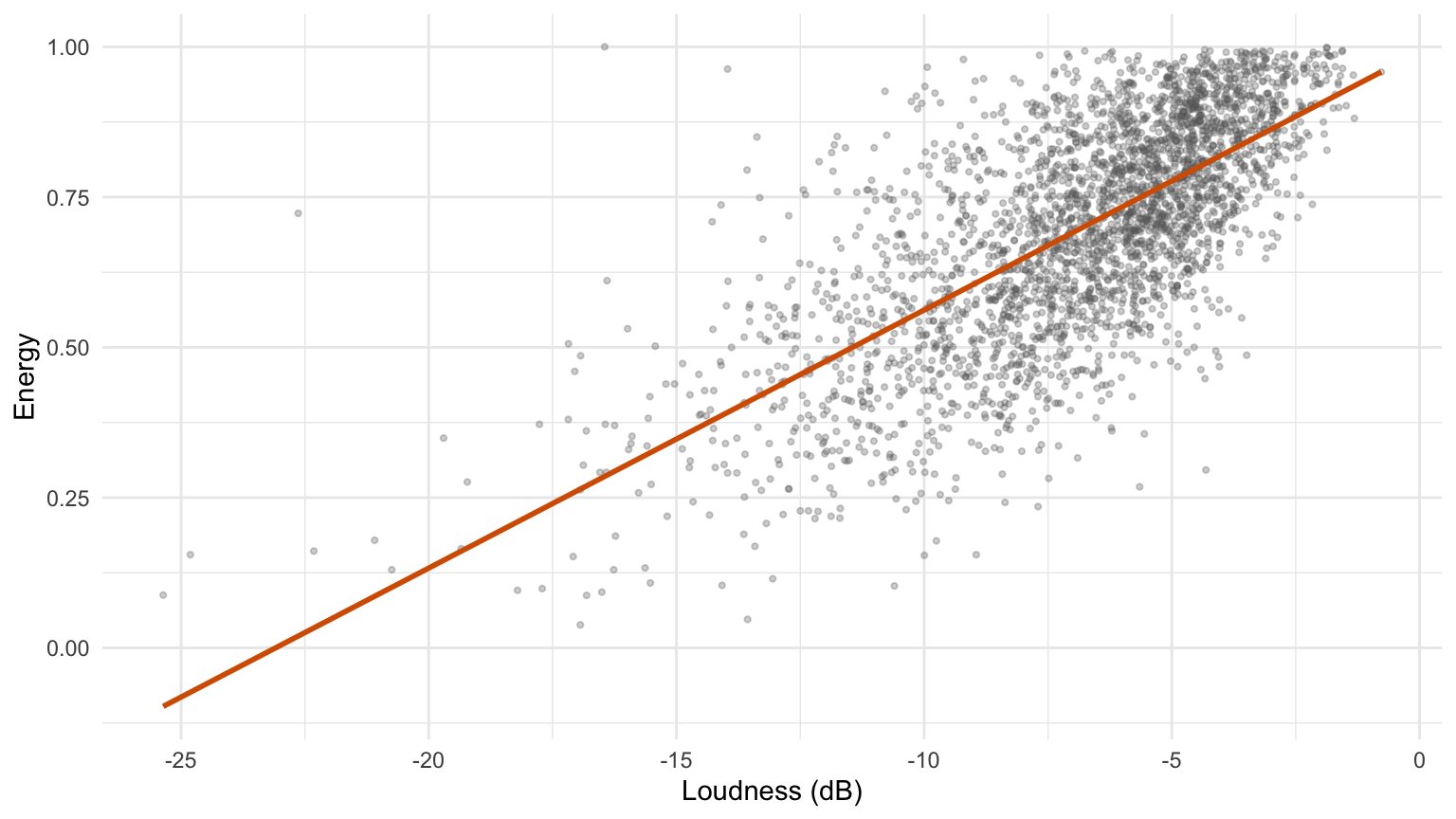
plot(M3, which = 1, main = "Residuals vs Fitted", caption = "")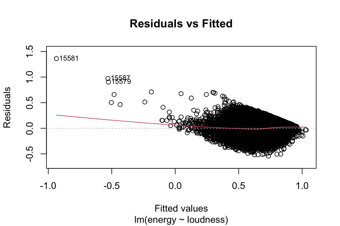
Questions:
Ramen ratings (TidyTuesday, June 4, 2019): star ratings (0 to 5) from The Ramen Rater. We keep three styles and three countries:
ramen <- read_csv("https://raw.githubusercontent.com/rfordatascience/tidytuesday/master/data/2019/2019-06-04/ramen_ratings.csv") |>
  filter(style %in% c("Pack", "Bowl", "Cup"),
         country %in% c("Japan", "South Korea", "United States"),
         !is.na(stars)) |>
  mutate(style = factor(style, levels = c("Bowl", "Cup", "Pack")),
         country = factor(country))

M4 <- lm(stars ~ style * country, data = ramen)
summary(M4)
Call:
lm(formula = stars ~ style * country, data = ramen)

Residuals:
    Min      1Q  Median      3Q     Max
-4.0074 -0.3705  0.0995  0.6615  1.6295

Coefficients:
                               Estimate Std. Error t value Pr(>|t|)
(Intercept)                     4.00743    0.07063  56.736  < 2e-16 ***
styleCup                       -0.26993    0.11924  -2.264 0.023781 *
stylePack                      -0.16897    0.09860  -1.714 0.086863 .
countrySouth Korea             -0.17761    0.12692  -1.399 0.161971
countryUnited States           -0.49524    0.12745  -3.886 0.000108 ***
styleCup:countrySouth Korea    -0.03766    0.21412  -0.176 0.860403
stylePack:countrySouth Korea    0.23963    0.15893   1.508 0.131891
styleCup:countryUnited States   0.12827    0.19095   0.672 0.501874
stylePack:countryUnited States  0.29022    0.16497   1.759 0.078804 .
---
Signif. codes:  0 '***' 0.001 '**' 0.01 '*' 0.05 '.' 0.1 ' ' 1

Residual standard error: 0.9607 on 1122 degrees of freedom
Multiple R-squared:  0.0369,    Adjusted R-squared:  0.03004
F-statistic: 5.374 on 8 and 1122 DF, p-value: 1.189e-06anova(M4)Analysis of Variance Table
Response: stars
Df Sum Sq Mean Sq F value Pr(>F)
style 2 13.00 6.4985 7.0409 0.0009145 ***
country 2 22.18 11.0915 12.0173 6.856e-06 ***
style:country 4 4.50 1.1251 1.2190 0.3009325
Residuals 1122 1035.57 0.9230
---
Signif. codes: 0 '***' 0.001 '**' 0.01 '*' 0.05 '.' 0.1 ' ' 1ramen |>
group_by(country, style) |>
summarise(mean_stars = mean(stars), .groups = "drop") |>
ggplot(aes(x = country, y = mean_stars, color = style, group = style)) +
geom_line(linewidth = 1.1) +
geom_point(size = 3) +
scale_color_manual(values = c("#0072B2", "#D55E00", "#009E73")) +
labs(x = "Country", y = "Mean stars", color = "Style")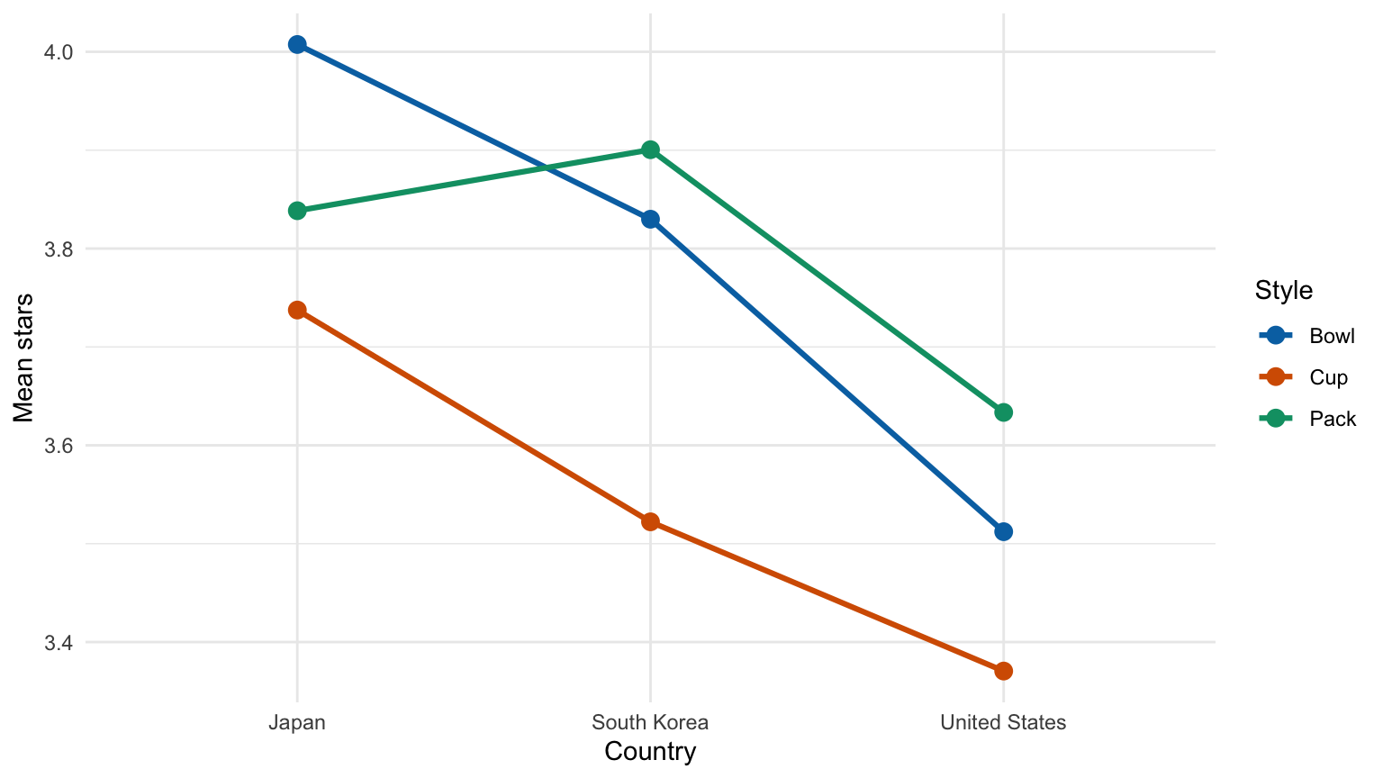
Questions:
Himalayan expeditions (TidyTuesday, September 22, 2020): we use members of Everest expeditions since 2000, excluding hired staff. success is TRUE if the person reached the summit.
everest <- read_csv("https://raw.githubusercontent.com/rfordatascience/tidytuesday/master/data/2020/2020-09-22/members.csv") |>
  # JUDGMENT CALL: Everest only, since 2000, excluding hired staff
  filter(peak_name == "Everest", year >= 2000, !hired, !is.na(age))
nrow(everest)
[1] 9139M5 <- glm(success ~ age, data = everest, family = binomial)
summary(M5)
Call:
glm(formula = success ~ age, family = binomial, data = everest)

Coefficients:
             Estimate Std. Error z value Pr(>|z|)
(Intercept)  0.697636   0.082725   8.433   <2e-16 ***
age         -0.020760   0.001984 -10.462   <2e-16 ***
---
Signif. codes:  0 '***' 0.001 '**' 0.01 '*' 0.05 '.' 0.1 ' ' 1

(Dispersion parameter for binomial family taken to be 1)

    Null deviance: 12624  on 9138  degrees of freedom
Residual deviance: 12512  on 9137  degrees of freedom
AIC: 12516

Number of Fisher Scoring iterations: 4exp(coef(M5))(Intercept) age
2.0089985 0.9794541 Questions:
M6 <- glm(success ~ age + oxygen_used, data = everest, family = binomial)
summary(M6)
Call:
glm(formula = success ~ age + oxygen_used, family = binomial,
    data = everest)

Coefficients:
                 Estimate Std. Error z value Pr(>|z|)
(Intercept)     -2.986736   0.161078 -18.542  < 2e-16 ***
age             -0.019934   0.002934  -6.794 1.09e-11 ***
oxygen_usedTRUE  4.958756   0.116946  42.402  < 2e-16 ***
---
Signif. codes:  0 '***' 0.001 '**' 0.01 '*' 0.05 '.' 0.1 ' ' 1

(Dispersion parameter for binomial family taken to be 1)

    Null deviance: 12623.8  on 9138  degrees of freedom
Residual deviance:  6714.5  on 9136  degrees of freedom
AIC: 6720.5

Number of Fisher Scoring iterations: 6exp(coef(M6)) (Intercept) age oxygen_usedTRUE
0.05045185 0.98026383 142.41651438 Questions:
oxygen_usedTRUE odds ratio in context. Can we conclude that oxygen causes success? Name one alternative explanation.