Influential Points, Regression Inference & ANOVA
Week 8
🐧 Penguins & Body Size
Last Tuesday we fit this model:
\[\widehat{\text{body mass}} = -5781 + 49.7 \times \text{flipper length} \quad R^2 = 75.9\%\]
But we noticed something: the residual plot had clusters. Our model fits okay, but it seems like something else is going on.
Today we’ll:
- Understand what makes an observation unusual or influential
- Learn to test whether our regression slope is really different from zero
- Discover how to compare three species at once using ANOVA
First: A Quick Review
Residual = actual − predicted = \(y_i - \hat{y}_i\)
Residual plots let us check whether:
- The linear model is appropriate (no curved pattern)
- Variance is roughly constant (no fan shape)
- There are unusual observations
Today’s question: What happens when a single penguin — or a single observation — has an outsized influence on our regression line?
Outliers in Regression
An outlier in regression is a point that doesn’t follow the general pattern.
Two types matter differently:
Outlier in y (large residual):
- Point falls far above or below the regression line
- Has a large residual
- May or may not change the slope much
Outlier in x (high leverage):
- Point falls far from the center of the x values
- Has high leverage — it can pull the line toward itself
A high-leverage point that actually does change the regression line is called an influential point.
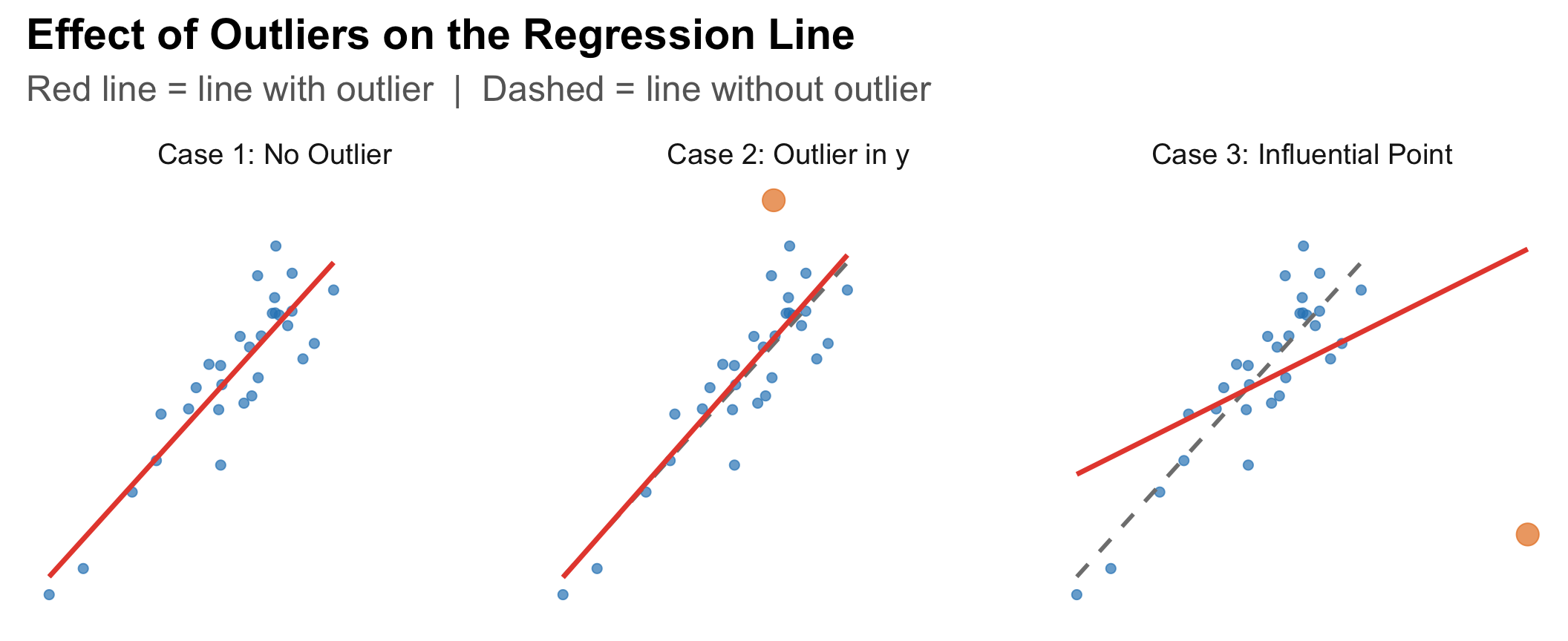
Influential Points: A Visual
![]()
Case 3 is the dangerous one. A single point can dramatically change the slope, intercept, and R².
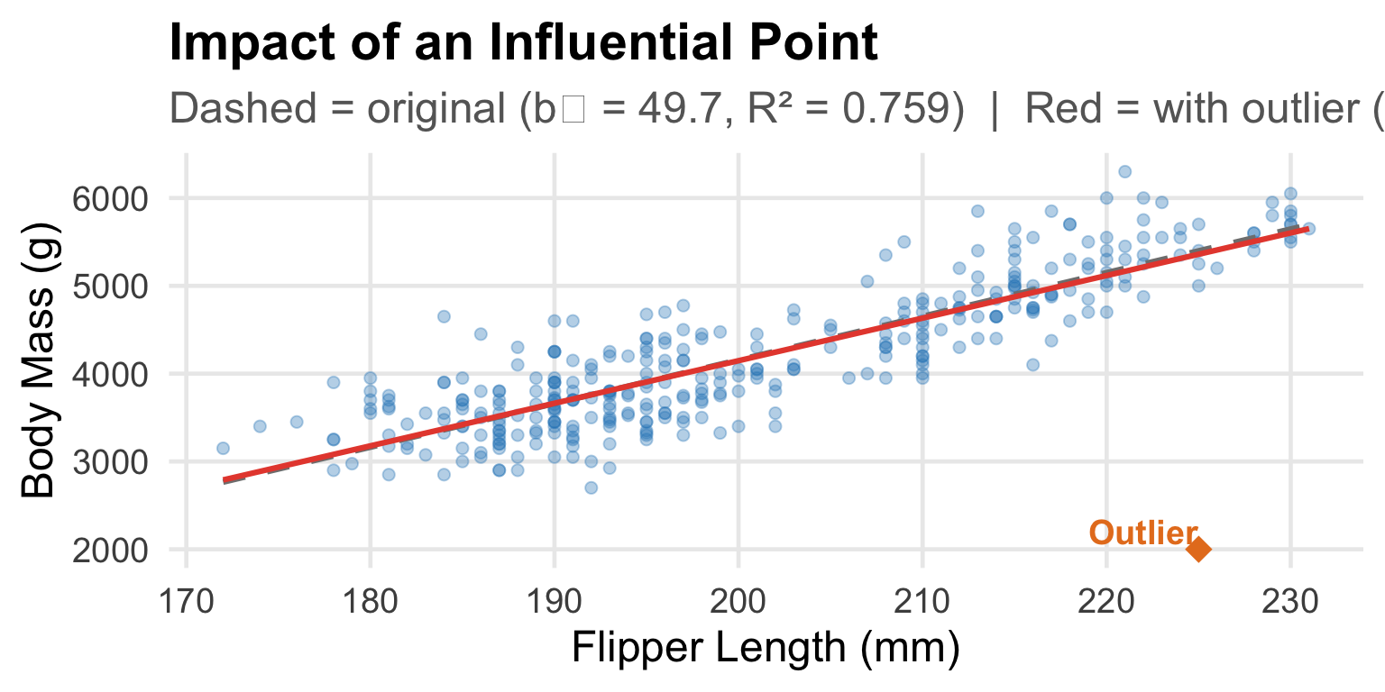
Spotting Influential Points: Penguin Example
What if we had one penguin with flipper = 225 mm but body mass = only 2000 g? (Much lighter than expected.)
![]()
One observation changed the slope from 49.7 to 48.5 g/mm and R² from 0.759 to 0.713.
What to Do With Outliers
Investigate first — is it a data entry error? A measurement mistake? Fix it if so.
Never delete just because it’s inconvenient — if it’s a real observation, it belongs in the analysis.
Report both analyses — fit the model with and without the influential point and report both. Let the reader see the effect.
Consider whether the model is misspecified — if there are many outliers, maybe a linear model isn’t the right choice at all.
In the penguin case: those clusters suggest we should include species as a variable — more on this after the break!
Think-Pair-Share #1
[Poll Everywhere — respond now!]
A researcher studying the relationship between caffeine intake (mg/day) and reaction time (ms) finds one participant who drinks 1200 mg/day (roughly 8 cups of coffee) — far more than anyone else in the study.
Discuss with your neighbor (2 min):
- Is this participant likely to have high leverage? Why?
- If this participant also has an unusually fast reaction time, would they be influential? What would happen to the slope?
- Should the researcher remove this participant from the analysis?
→ Vote on Q3: Remove the participant? Yes / No / Investigate first
Regression Inference: Is the Slope Real?
We found a slope of 49.69 g/mm for penguins. But could this just be sampling variability?
Hypotheses:
\(H_0: \beta_1 = 0\) (no linear relationship between flipper length and body mass in the population)
\(H_a: \beta_1 \neq 0\) (there IS a linear relationship)
We test this using the t-statistic from the R output:
\[t = \frac{b_1 - 0}{SE(b_1)} = \frac{49.69}{1.52} = 32.72\]
Reading the R Output
Call:
lm(formula = body_mass_g ~ flipper_length_mm, data = penguins_clean)

Residuals:
     Min       1Q   Median       3Q      Max
-1058.80  -259.27   -26.88   247.33  1288.69

Coefficients:
                   Estimate Std. Error t value Pr(>|t|)
(Intercept)       -5780.831    305.815  -18.90   <2e-16 ***
flipper_length_mm    49.686      1.518   32.72   <2e-16 ***
---
Signif. codes:  0 '***' 0.001 '**' 0.01 '*' 0.05 '.' 0.1 ' ' 1

Residual standard error: 394.3 on 340 degrees of freedom
Multiple R-squared:  0.759, Adjusted R-squared:  0.7583
F-statistic:  1071 on 1 and 340 DF,  p-value: < 2.2e-16
What the p-value Tells Us
p-value < 0.0001:
If there were truly no relationship between flipper length and body mass in the population, the probability of observing a slope as extreme as 49.69 (or more extreme) just by chance is essentially zero.
Conclusion:
There is very strong evidence of a statistically significant positive linear relationship between flipper length and body mass in penguins (slope = 49.69 g/mm, t = 32.72, p < 0.001).
A 95% confidence interval for the slope: approximately \(49.69 \pm 2(1.52) = (46.6,\ 52.7)\) g/mm.
We’re 95% confident that each additional mm of flipper length is associated with a 46.6 to 52.7 gram increase in body mass.
Conditions for Regression Inference
Remember LINE — but now we’re more careful:
Linearity — verified by scatterplot and residual plot ✅
Independence — penguins measured once, random sample ✅
Normal residuals — check histogram of residuals (roughly bell-shaped) ✅
Equal variance — residual plot shows roughly constant spread ✅
When these conditions are met, the t-test on the slope is valid. If not — the p-value and confidence intervals can’t be trusted.
Think-Pair-Share #2
[Poll Everywhere — respond now!]
From the R output:
| (Intercept) |
-5780.8314 |
305.8145 |
-18.9031 |
0 |
| flipper_length_mm |
49.6856 |
1.5184 |
32.7222 |
0 |
Discuss with your neighbor (2 min):
- A student says: “R² = 0.759, so the model is wrong 24.1% of the time.” Is this correct? How would you fix this statement?
- What does the standard error of 1.52 tell us about our estimate of the slope?
- Write one sentence interpreting the slope in plain biological language.
→ Share your interpretation of the slope on Poll Everywhere
☕ BREAK — 10 minutes
Coming up after the break:
We’ve been comparing two quantities. But what if we want to compare three species of penguins simultaneously? Just doing three separate t-tests creates a serious problem…
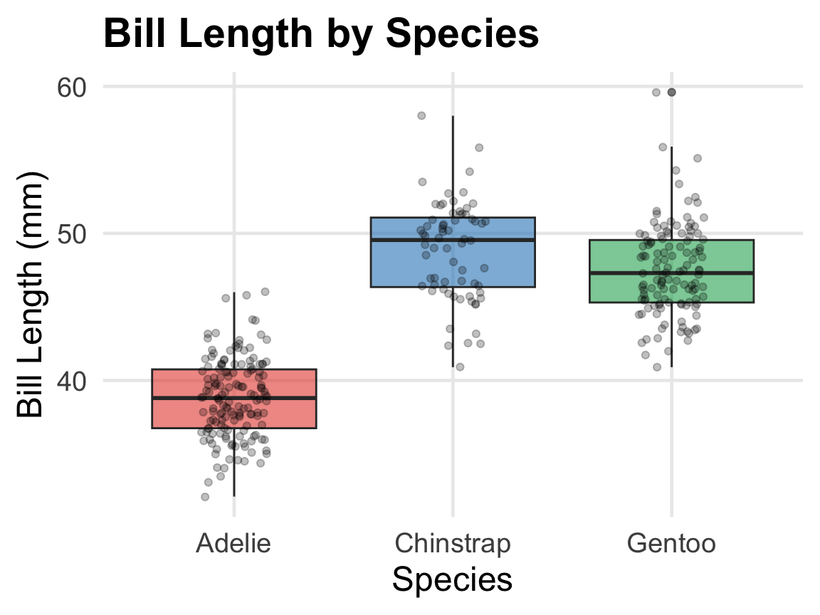
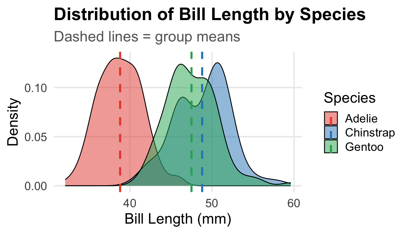
A New Question: Do Species Differ?
The three penguin species — Adelie, Chinstrap, and Gentoo — live on different islands and have evolved differently.
Question: Do the three species have different mean bill lengths?
| Adelie |
151 |
38.8 |
2.7 |
| Chinstrap |
68 |
48.8 |
3.3 |
| Gentoo |
123 |
47.5 |
3.1 |
There appear to be differences — but could these arise from sampling variability alone?
Why Not Just Do Multiple t-Tests?
We have 3 groups → 3 possible comparisons:
- Adelie vs. Chinstrap
- Adelie vs. Gentoo
- Chinstrap vs. Gentoo
If we use α = 0.05 for each test, the probability of making at least one Type I error is:
\[P(\text{at least one false positive}) = 1 - (1-0.05)^3 = 1 - 0.857 = 0.143\]
14.3% chance of a false positive — nearly 3× our intended error rate!
With 10 groups (45 comparisons): \(1 - (0.95)^{45} = 90\)% chance of a false positive.
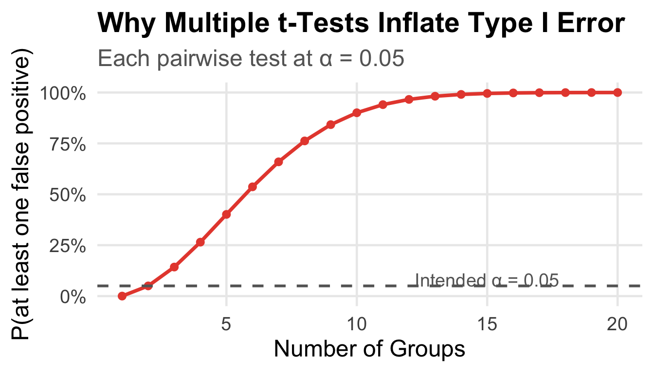
The Multiple Testing Problem
![]()
ANOVA (Analysis of Variance) tests all groups simultaneously with one test, keeping Type I error exactly at α.
The Logic of ANOVA
ANOVA asks: Is the variability between groups larger than the variability within groups?
![]()
The group means are far apart relative to the spread within each group → strong signal.
The F-Statistic
ANOVA summarizes this as the F-statistic:
\[F = \frac{\text{Mean Square Between groups (MSG)}}{\text{Mean Square Within groups (MSE)}} = \frac{\text{Signal}}{\text{Noise}}\]
- Large F → between-group variation is large relative to within-group variation → evidence against H₀
- F ≈ 1 → between ≈ within → no evidence groups differ
Hypotheses:
\[H_0: \mu_{\text{Adelie}} = \mu_{\text{Chinstrap}} = \mu_{\text{Gentoo}}\]
\[H_a: \text{At least one mean is different}\]
ANOVA Output from R
             Df Sum Sq Mean Sq F value Pr(>F)
species       2   7194    3597   410.6 <2e-16 ***
Residuals   339   2970       9
---
Signif. codes:  0 '***' 0.001 '**' 0.01 '*' 0.05 '.' 0.1 ' ' 1
Reading the table:
Df |
Degrees of freedom (groups − 1 = 2; total − groups = 339) |
Sum Sq |
Sum of squared deviations |
Mean Sq |
Sum Sq ÷ Df |
F value |
F = 3597 ÷ 8.8 = 410.6 |
Pr(>F) |
p-value < 2×10⁻¹⁶ |
Interpreting the ANOVA Output
F = 410.6, df = 2 and 339, p < 0.001
Decision: p < 0.001, so we reject H₀ at any reasonable α.
Conclusion in context:
There is very strong statistical evidence that at least one penguin species has a different mean bill length than the others (F = 410.6, df = 2 and 339, p < 0.001).
Important caveat: ANOVA only tells us that at least one mean differs. It does not tell us which pairs differ. For that, we’d need post-hoc tests (e.g., Tukey’s HSD) — a topic for future courses!
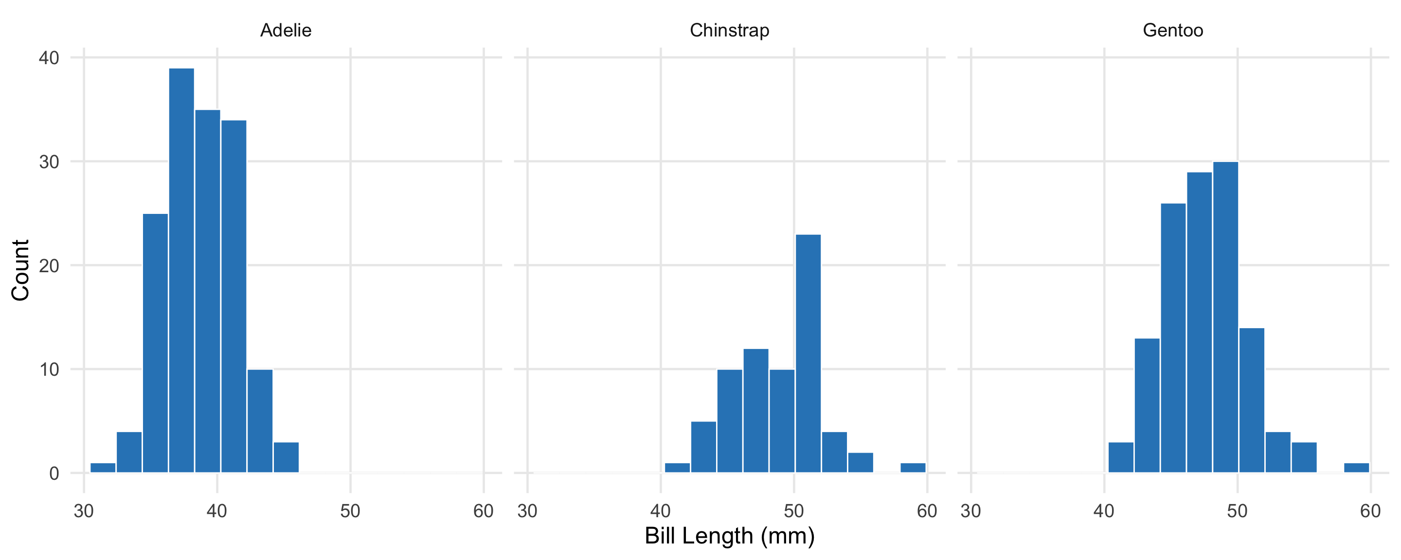
Conditions for ANOVA
Like the t-test, ANOVA requires checking conditions:
1. Independence
Observations within and across groups must be independent (study design)
2. Approximate normality
The response should be roughly normal within each group, or n large enough for CLT to apply
3. Equal variance
SD should be roughly similar across groups. Largest SD (3.3) < twice the smallest (2.7)
| Adelie |
151 |
2.7 |
| Chinstrap |
68 |
3.3 |
| Gentoo |
123 |
3.1 |
![]()
Think-Pair-Share #3
[Poll Everywhere — respond now!]
A health researcher wants to compare mean cholesterol levels across four diet groups: vegan, vegetarian, pescatarian, and omnivore. She plans to run six pairwise t-tests.
Discuss with your neighbor (2 min):
- What is the probability of at least one false positive if she uses α = 0.05 for all 6 tests? (Hint: \(1 - 0.95^6\))
- What should she use instead? What are the hypotheses for this test?
- She runs ANOVA and gets F = 3.2, p = 0.027. What can she conclude — and what can she not conclude?
→ Answer Q1 (the probability) on Poll Everywhere
Week 8 Summary: Putting It All Together
The penguins taught us a lot this week:
Tuesday:
- Scatterplots visualize two numerical variables
- Correlation (r) quantifies linear association
- Correlation ≠ causation
- Regression predicts; slope and intercept have specific interpretations
- R² measures proportion of variability explained
- Residual plots check model assumptions
Thursday:
- Outliers vs. influential points — leverage matters
- Regression inference: t-test on slope from R output
- ANOVA: comparing 3+ group means without inflating Type I error
- F-statistic = signal/noise ratio
The Big Picture
We’ve now covered the major tools of statistical inference:
| One mean |
One-sample t-test |
| Before vs. after, same subjects |
Paired t-test |
| Two independent groups |
Two-sample t-test |
| Three or more groups |
ANOVA |
| Two numerical variables |
Correlation & Regression |
These aren’t separate techniques — they’re all part of one framework: asking whether what we observe could plausibly be due to chance alone.
Reminders
HW7 covers this week’s material — due next week
DSA8 last one in discussion sections next week!
Next week: categorical data: proportions and independence
Great work this week, Statistical Detectives! 🐧🔍