Scatterplots, Correlation & Linear Regression

Week 8

🐧 Penguins & Body Size

A question from evolutionary biology:

Can we predict how heavy a penguin is just by measuring its flipper?

Researchers at Palmer Station, Antarctica measured 344 penguins across three species:

• Flipper length (mm)
• Body mass (g)
• Bill length and depth (mm)
• Species, island, sex

Today we’ll use this dataset to understand how two numerical variables relate — and how to use one to predict the other.

The Data: One Snapshot

A random sample of 6 penguins from the dataset:

Flipper Length (mm)	Body Mass (g)
191	4150
190	3400
230	5700
190	3700
209	4600
190	4250

Just looking at numbers is hard. We need a visualization.

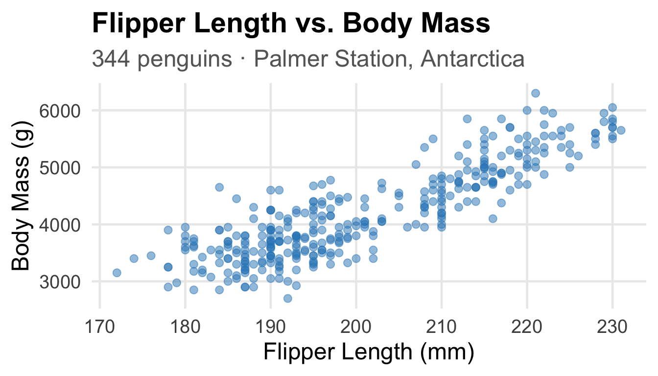
Review: The Scatterplot

A scatterplot displays the relationship between two numerical variables.

• Each point = one observation (one penguin)
• x-axis = explanatory variable (flipper length)
• y-axis = response variable (body mass)

What to Look for in a Scatterplot

When describing a scatterplot, always comment on:

1. Direction — Does the relationship go up or down?

As flipper length increases, body mass tends to increase (positive)

2. Form — Is the pattern linear or curved?

The relationship appears roughly linear

3. Strength — How tightly do the points cluster around the pattern?

Points cluster fairly closely → moderately strong

4. Outliers — Any unusual points?

A few points fall away from the main trend

Think-Pair-Share #1

[Poll Everywhere — respond now!]

Look at this scatterplot description:

“As daily average temperature increases, hot chocolate sales decrease. The relationship is fairly linear and strong, with one outlier on a very cold day.”

Discuss with your neighbor (2 min):

1. What is the direction, form, and strength?
2. Which is the explanatory variable? Which is the response variable?
3. Can we conclude that cold weather causes people to buy more hot chocolate? Why or why not?

→ Report your answer to Q3 on Poll Everywhere

Review: Correlation

We can measure the strength and direction of a linear relationship with the correlation coefficient r.

\[r = \frac{1}{n-1}\sum_{i=1}^{n}\left(\frac{x_i - \bar{x}}{s_x}\right)\left(\frac{y_i - \bar{y}}{s_y}\right)\]

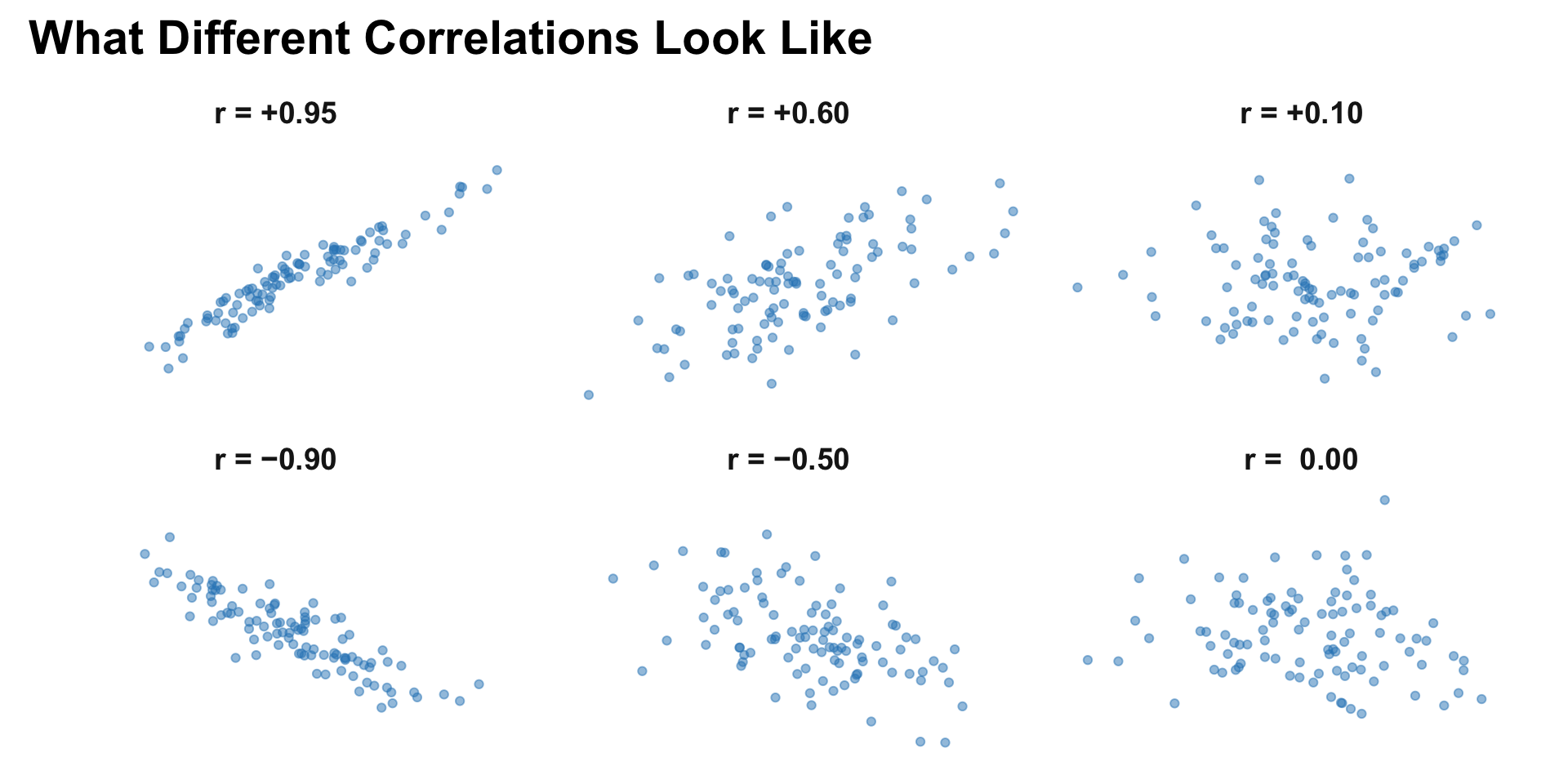
Properties of r:

• Always between −1 and +1
• r = +1: perfect positive linear relationship
• r = −1: perfect negative linear relationship
• r = 0: no linear relationship
• Sign tells us direction; magnitude tells us strength

Correlation: Visual Guide

For the penguins: Flipper length vs. body mass gives r = 0.87

Interpretation: Strong, positive linear relationship between flipper length and body mass.

⚠️ Correlation ≠ Causation

r = 0.87 means flipper length and body mass are strongly associated — but does longer flippers cause heavier penguins?

Possible explanations for an association:

1. X causes Y (flipper length drives body mass)
2. Y causes X (heavier penguins develop longer flippers)
3. Lurking variable: a third variable drives both (e.g., age or species)
4. Coincidence (unlikely with r = 0.87, but possible with small n)

Famous spurious correlations:

• Per capita cheese consumption correlates with deaths by bedsheet tangling (r = 0.95!)
• Nicolas Cage films per year correlates with pool drownings (r = 0.67!)
• Other ridiculous examples: https://www.tylervigen.com/spurious-correlations

Think-Pair-Share #2

[Poll Everywhere — respond now!]

Researchers find that students who eat breakfast regularly have higher GPAs (r = 0.45, p < 0.001).

Discuss with your neighbor (2 min):

1. Is this correlation positive or negative? Strong or weak?
2. A journalist writes: “Eating breakfast improves academic performance.” Is this conclusion justified? What’s missing?
3. Name one lurking/confounding variable that might explain this association without breakfast directly causing better grades.

→ Report your confounding variable on Poll Everywhere

Linear Regression

Correlation tells us how strongly two variables are related.

Regression gives us a line to describe or predict the response from the explanatory variable.

The least squares regression line minimizes the sum of squared residuals:

\[\hat{y} = b_0 + b_1 x\]

where:

• \(\hat{y}\) = predicted response
• \(b_0\) = y-intercept
• \(b_1\) = slope

For our penguins:

\[\widehat{\text{body mass}} = -5781 + 49.7 \times \text{flipper length}\]

Calculating the Regression Line

The least squares formulas for slope and intercept:

Slope:

\[b_1 = r \cdot \frac{s_y}{s_x}\]

where \(r\) is the correlation, \(s_y\) is the SD of the response, and \(s_x\) is the SD of the explanatory variable.

Intercept:

\[b_0 = \bar{y} - b_1 \bar{x}\]

The line always passes through the point \((\bar{x},\ \bar{y})\) — the means of both variables.

For our penguins:

\[b_1 = 0.87 \cdot \frac{802}{44} = 49.7 \text{ g/mm} \qquad b_0 = 4202 - 49.7 \times 200 = -5781 \text{ g}\]

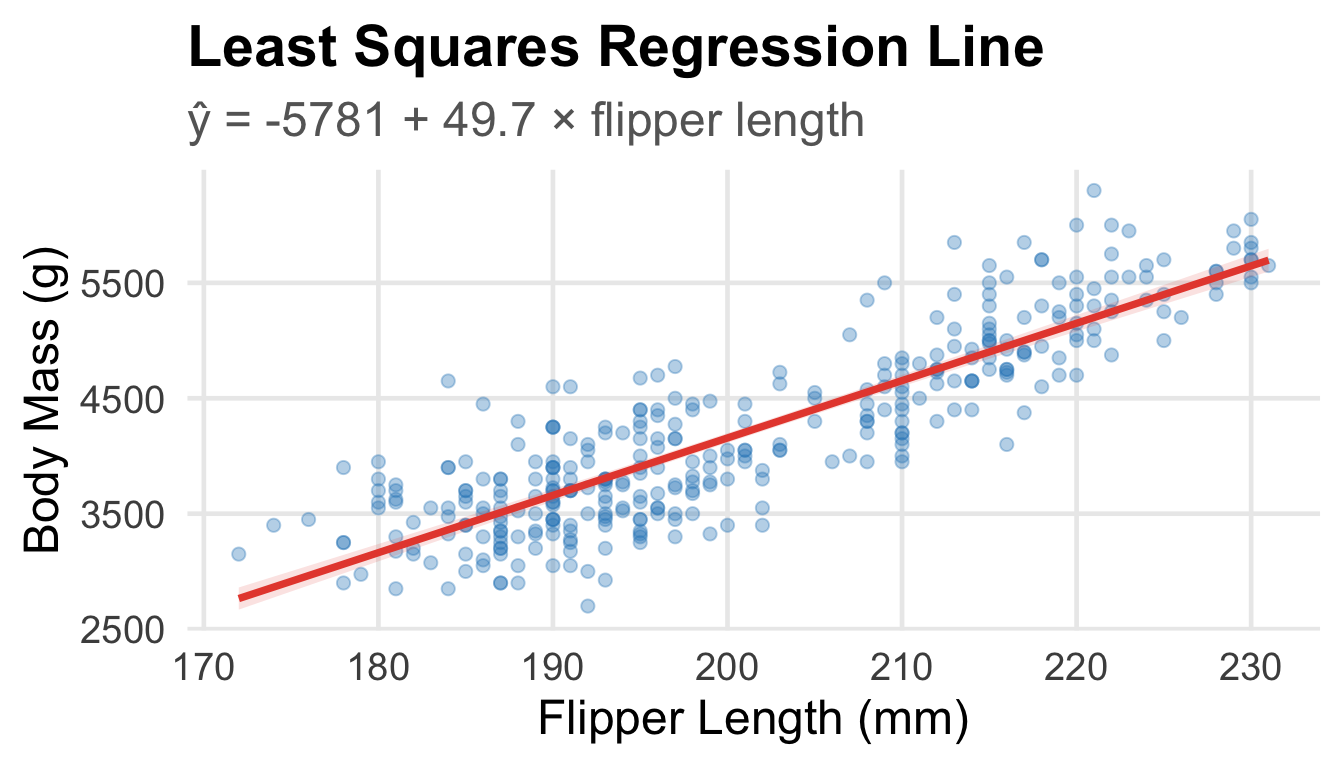
Interpreting the Regression Line

Slope (b₁ = 49.7): For each additional 1 mm of flipper length, predicted body mass increases by 49.7 grams, on average.

Intercept (b₀ = -5781): A penguin with flipper length = 0 mm would be predicted to weigh -5781 grams — 🚨 not meaningful, just a mathematical anchor.

Making Predictions

\[\widehat{\text{body mass}} = -5781 + 49.7 \times \text{flipper length}\]

Example: A penguin has a flipper length of 200 mm. Predict its body mass.

\[\hat{y} = -5781 + 49.7 \times 200 = 4159 \text{ g}\]

⚠️ Extrapolation warning:

The penguin data ranges from flipper lengths of 172–231 mm.

Predicting for flipper = 100 mm or flipper = 300 mm is extrapolation — we have no data there and the linear pattern may not hold!

R Output: The Full Picture

Call:
lm(formula = body_mass_g ~ flipper_length_mm, data = penguins_clean)

Residuals:
     Min       1Q   Median       3Q      Max 
-1058.80  -259.27   -26.88   247.33  1288.69 

Coefficients:
                   Estimate Std. Error t value Pr(>|t|)    
(Intercept)       -5780.831    305.815  -18.90   <2e-16 ***
flipper_length_mm    49.686      1.518   32.72   <2e-16 ***
---
Signif. codes:  0 '***' 0.001 '**' 0.01 '*' 0.05 '.' 0.1 ' ' 1

Residual standard error: 394.3 on 340 degrees of freedom
Multiple R-squared:  0.759, Adjusted R-squared:  0.7583 
F-statistic:  1071 on 1 and 340 DF,  p-value: < 2.2e-16

What does R² = 0.759 tell us?

Interpreting R²

R² (R-squared) = the proportion of variability in the response variable explained by the model.

R² = 0.759 means:

75.9% of the variability in penguin body mass is explained by flipper length.

The remaining 24.1% is due to other factors (species, sex, diet, age, etc.)

Relationship to r:

\[R^2 = r^2 = (0.87)^2 = 0.7569 \approx 0.759\]

For simple linear regression, R² is literally the correlation squared!

☕ BREAK — 10 minutes

While you rest, think about:

We’ve predicted body mass from flipper length. But how well does our line actually fit? How do we check?

See you in 10!

Residuals: How Far Off Are We?

The residual for each observation is the difference between the actual and predicted values:

\[e_i = y_i - \hat{y}_i\]

Example:

• Penguin with flipper = 200 mm, actual body mass = 4800 g
• Predicted: \(\hat{y} = -5781 + 49.7(200) = 4159\) g
• Residual: \(e = 4800 - 4159 = 641\) g

A positive residual → actual value is above the line (we underpredicted)

A negative residual → actual value is below the line (we overpredicted)

The least squares line is chosen to make the sum of squared residuals as small as possible.

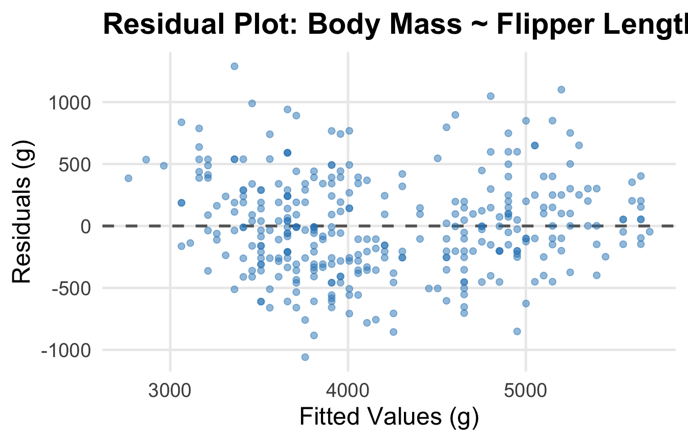
Residual Plots: Checking the Model

To check whether a linear model is appropriate, we plot residuals vs. fitted values.

What we want to see: No pattern — random scatter around zero.

Reading Residual Plots

✅ Good: Random scatter around zero

→ Linear model is appropriate; constant variance

❌ Problem: Curved pattern

→ The relationship is not truly linear; consider transformations

❌ Problem: Fan shape (variance increases)

→ Constant variance assumption is violated

❌ Problem: Outliers (one or two extreme points)

→ Investigate those observations carefully

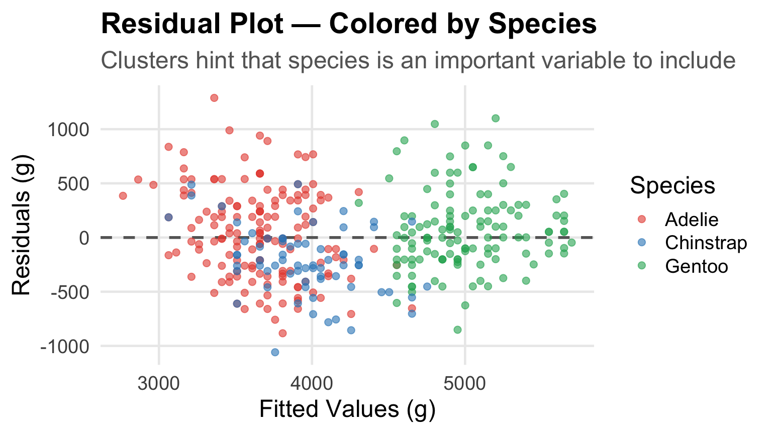
Residual Plot for Penguins

Interpretation: Clusters by species reveal that mixing three species creates structure in the residuals — species is a lurking variable!

Think-Pair-Share #3

[Poll Everywhere — respond now!]

A researcher fits a linear regression of plant height (cm) on amount of fertilizer (g). The residual plot shows a clear U-shaped curve.

Discuss with your neighbor (2 min):

1. What does this U-shape in the residual plot tell us?
2. Is the linear model appropriate here? What would you recommend?
3. In the penguin data, we noticed clusters in the residual plot. What variable might be creating these clusters?

→ Report your answer to Q3 on Poll Everywhere

Conditions for Linear Regression

For regression to be valid (especially for inference), we need:

Linearity — the relationship between x and y is linear (check scatterplot)

Independence — observations are independent of each other (study design)

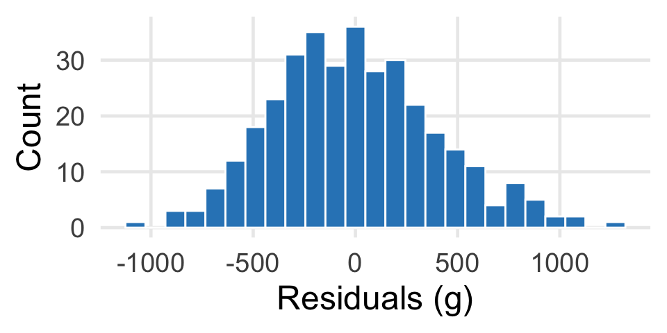
Normal residuals — residuals are approximately normally distributed (check histogram of residuals)

Equal variance — residuals have roughly constant spread (check residual plot)

Remember the acronym: LINE

Today’s Summary

1. Scatterplots visualize the relationship between two numerical variables — describe direction, form, strength, and outliers

2. Correlation (r) quantifies linear association: ranges from −1 to +1

3. Correlation ≠ Causation — association could be due to lurking variables

4. Regression line (\(\hat{y} = b_0 + b_1 x\)) predicts the response from the explanatory variable

5. Slope: change in predicted ŷ per 1-unit increase in x; Intercept: predicted ŷ when x = 0

6. R²: proportion of variability in y explained by the model

7. Residual plots: check for linearity and equal variance assumptions

Looking Ahead: Thursday

Next class we cover:

• Outliers and influential points — what happens when we have unusual observations?
• Regression inference — testing whether the slope is really different from zero
• Reading full R output for regression
• ANOVA — comparing means across three or more groups

The penguins will be back! We’ll compare bill length across all three species.