Difference in means: -2.7 mmHgStandard error: 0.88 mmHgt-statistic: -3.08 df: 150 p-value: < 0.001STAT 7 - Winter 2026
Today’s Plan
The DASH Diet Study (Appel et al., 1997, NEJM)
We analyzed a paired design:
Today: How do we compare the DASH diet to OTHER diets?
Three independent groups (different people in each):
Key difference from Tuesday:
Research Question: Does the DASH diet reduce blood pressure more than the Fruits & Vegetables diet?
Summary statistics (change in systolic BP from baseline):
Note: Negative values indicate BP decreased (good!)
Independent samples - Different people in each diet group
Let μ₁ = mean BP change for DASH diet
Let μ₂ = mean BP change for F&V diet
Why two-sided? Though we expect DASH to be better, we test for any difference.
\[t = \frac{(\bar{x}_1 - \bar{x}_2) - (\mu_1 - \mu_2)}{\sqrt{\frac{s_1^2}{n_1} + \frac{s_2^2}{n_2}}}\]
Where:
Simple approximation: \(df = \min(n_1 - 1, n_2 - 1)\)
Better approximation (Welch’s):
\[df = \frac{(s_1^2/n_1 + s_2^2/n_2)^2}{(s_1^2/n_1)^2/(n_1-1) + (s_2^2/n_2)^2/(n_2-1)}\]
Statistical software uses Welch’s method automatically.
For our example: df ≈ 150 (using simpler method)
Difference in means: -2.7 mmHgStandard error: 0.88 mmHgt-statistic: -3.08 df: 150 p-value: < 0.001Decision: p < 0.001, reject H₀
Conclusion: The DASH diet reduces blood pressure significantly more than the Fruits & Vegetables diet alone (additional reduction of 2.7 mmHg, p < 0.001).
Statistical result: p < 0.001 - highly significant
Practical significance:
The bigger picture:
All three differ significantly from each other!
\[(\bar{x}_1 - \bar{x}_2) \pm t^* \times \sqrt{\frac{s_1^2}{n_1} + \frac{s_2^2}{n_2}}\]
For 95% CI with large df, \(t^* \approx 1.96\):
95% CI: (-4.42, -0.98) mmHgInterpretation: We’re 95% confident that the DASH diet reduces blood pressure between 0.98 and 4.42 mmHg more than the F&V diet.
Note: Entire interval is negative (favoring DASH)
Comparison: Control diet showed 0.9 mmHg reduction. DASH showed 5.5 mmHg reduction. Difference = 4.6 mmHg (p < 0.001).
The DASH study meets all conditions!
Break Time! ☕ 5-minute break
Stretch, grab water, chat with neighbors!
We’ll resume with conditional probability.
Based on DASH results, researchers want to design a new study:
Question: Can a modified DASH diet be effective in adolescents with pre-hypertension?
Imagine planning this new dietary intervention study…
Power = Probability of correctly rejecting H₀ when Hₐ is true
In other words: Probability of detecting a real effect when it exists
| H₀ is TRUE | H₀ is FALSE (Hₐ is TRUE) | |
|---|---|---|
| Reject H₀ | Type I Error (False Positive) - Probability = α | Correct! (True Positive) - Probability = 1-β (Power) |
| Fail to Reject H₀ | Correct (True Negative) - Probability = 1-α | Type II Error (False Negative) - Probability = β |
Power = 1 - β = Probability of detecting a true effect
Typical goal: Power ≥ 80% (sometimes 90%)
Power depends on:
Scenario: Researchers want to test a simplified DASH-style diet in adolescents.
Why n = 50? Budget constraints for this pilot study
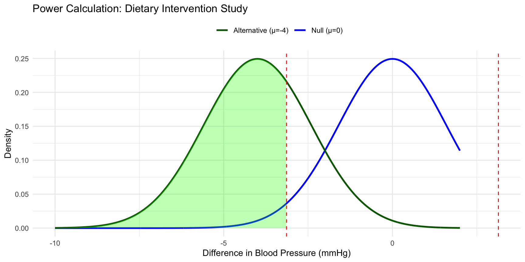
Null distribution (H₀: no difference):
Alternative distribution (Hₐ: difference = -4):
Rejection region: |difference| > 1.96 × 1.60 = 3.14 mmHg
Green area = Power = P(Reject H₀ | Hₐ is true) ≈ 71%
Step 1: Find rejection region for H₀
Step 2: Calculate probability under Hₐ (when true difference = -4)
Power ≈ 71% - Better than our earlier example, but could be higher.
Interpretation: If the diet truly reduces BP by 4 mmHg, there’s a 71% chance this study will detect it.
The dietary intervention study has 71% power with n=50 per group to detect a 4 mmHg reduction.
Target: 80% power to detect Δ = 4 mmHg reduction
Key insight: Rejection region is always 1.96 SE from 0. We need the alternative distribution far enough left that 80% falls in the rejection region.
This requires: \(0.84 \times SE + 1.96 \times SE = 4\)
Where 0.84 is the z-score for 80th percentile (for 80% power)
\[2.8 \times SE = 4\]
\[SE = \frac{4}{2.8} = 1.43\]
Since \(SE = \sqrt{\frac{\sigma_1^2}{n} + \frac{\sigma_2^2}{n}} = \sqrt{\frac{2\sigma^2}{n}}\) with σ = 8:
\[\sqrt{\frac{2 \times 8^2}{n}} = 1.43\]
\[n = \frac{2 \times 8^2}{1.43^2} = 63\] participants per group
Conclusion: Need 63 adolescents in each diet group for 80% power.
For comparing two means with equal n per group:
\[n = \frac{(\sigma_1^2 + \sigma_2^2)(z_{1-\alpha/2} + z_{1-\beta})^2}{\Delta^2}\]
Where:
Always round UP!
Using the formula for our dietary study:
\[n = \frac{(8^2 + 8^2)(1.96 + 0.84)^2}{4^2}\]
\[n = \frac{128 \times (2.8)^2}{16} = \frac{128 \times 7.84}{16} = 62.7\]
Round up to n = 63 per group ✓
This matches our earlier calculation!
A nutrition researcher wants to test omega-3 supplementation on inflammation markers.
Calculate: How many participants needed per group?
\[n = \frac{(12^2 + 12^2)(1.96 + 1.28)^2}{8^2}\]
Where:
\[n = \frac{2 \times 144 \times (3.24)^2}{64} = \frac{288 \times 10.50}{64} = 47.25\]
Answer: Need 48 participants per group (supplement vs. placebo)
This is a modest sample size - omega-3 studies are feasible!
Researchers want to study the DASH diet in older adults (65+). They can afford to enroll 40 participants total (20 per group). Previous data shows σ = 10 mmHg, and they want to detect Δ = 5 mmHg.
Original DASH trial (1997):
Impact:
Key lesson: Good study design with proper power analysis leads to impactful science!
Why not always use huge samples for 99% power?
Standard practice: Target 80-90% power
| To Increase Power: | Effect on Study: |
|---|---|
| Increase sample size (n) | More expensive, takes longer |
| Study larger effect sizes (Δ) | May not match research question |
| Reduce variability (σ) | Better measurement, stricter inclusion |
| Increase α | More Type I errors - usually not done |
Bottom line: Sample size is usually the only practical lever
Bottom line: Invest time in planning. The DASH researchers did, and it changed nutrition guidelines!
Next week (Week 8):
Before next class: