From Samples to Populations
Sampling Distributions and the Central Limit Theorem
Today’s Goals
- Understand the difference between population parameters and sample statistics
- Describe what a sampling distribution is
- State the Central Limit Theorem in plain language
- Connect these ideas to inference: making conclusions about populations from samples
Sleep Study
A researcher wants to know the average sleep duration of college students per day.
Population: All college students
Parameter: Average sleep hours (μ) per day
Sample: 100 students surveyed -> random sample
Statistic: Sample mean = 6.8 hours (\(\bar{x}\))
Key Question: How confident can we be that 6.8 hours represents the true population average?
Think-Pair-Share #1
Scenario: You want to estimate the average mercury level in anchovies fished in the Monterey Bay.
You obtain 25 anchovies using a random sample from local fisheries and test them, finding an average mercury level of 0.055 ppm.
Questions to discuss (2 minutes):
- What is the population? What is the parameter of interest?
- What is the sample? What is the statistic?
- If you tested a different set of 25 anchovies, would you get exactly 0.055 ppm again? Why or why not?
Quick Report: Answer Poll with your opinion ✋
Population vs. Sample
Population
- All individuals/units of interest
- Parameter: Fixed (but unknown) value
- Examples: μ (mean), p (proportion)
Sample
- Subset of the population
- Statistic: Varies from sample to sample
- Examples: \(\bar{x}\) (sample mean), \(\hat{p}\) (sample proportion)
We use statistics to estimate parameters, but statistics vary due to sampling variability.
Sampling Variability: A Demonstration
Let’s conduct an experiment together!
Activity: Estimate the average height in cms in this class
- Enter your data: Go to https://bit.ly/3Zo5xoc and enter your height (in cms)
- Watch what happens: I’ll randomly sample 20 students and calculate their average height
- Repeat: I’ll take another random sample of 20 different students
- Compare: Will we get the same average both times?
What we’ll observe: Different samples → different sample means (sampling variability)
Even from the same population, different samples give different results!
What is a Sampling Distribution?
- The sampling distribution shows what values a statistic (like \(\bar{x}\)) can take across all possible samples
- It’s the distribution of the statistic, not the distribution of individuals
- Shows us the pattern of sampling variability
Example: If we took 1000 different samples of 25 fish, we’d get 1000 different sample means. The sampling distribution shows how those means are distributed.
Think-Pair-Share #2
Scenario: You’re studying bird migration distances. You take samples of 50 birds each.
Sample 1: \(\bar{x}_1\) = 2,430 km
Sample 2: \(\bar{x}_2\) = 2,510 km
Sample 3: \(\bar{x}_3\) = 2,465 km
Questions to discuss (2 minutes):
- Why are these sample means different?
- What would happen to the variation between sample means if you sampled 200 birds instead of 50?
- If you took hundreds of samples, what pattern might you see in the sample means?
Quick Report: What affects how much sample means vary? ✋
The Central Limit Theorem (CLT)
In plain language:
When you take sufficiently large random samples from any population, the sampling distribution of the sample mean will be approximately normal (bell-shaped).
- Center: The mean of the sampling distribution equals the population mean μ
- Spread: The standard deviation (standard error) = \(\frac{\sigma}{\sqrt{n}}\)
- Shape: Approximately normal if n is large enough (usually n ≥ 30)
Why the CLT is Powerful
Population distribution
(can be any shape!)
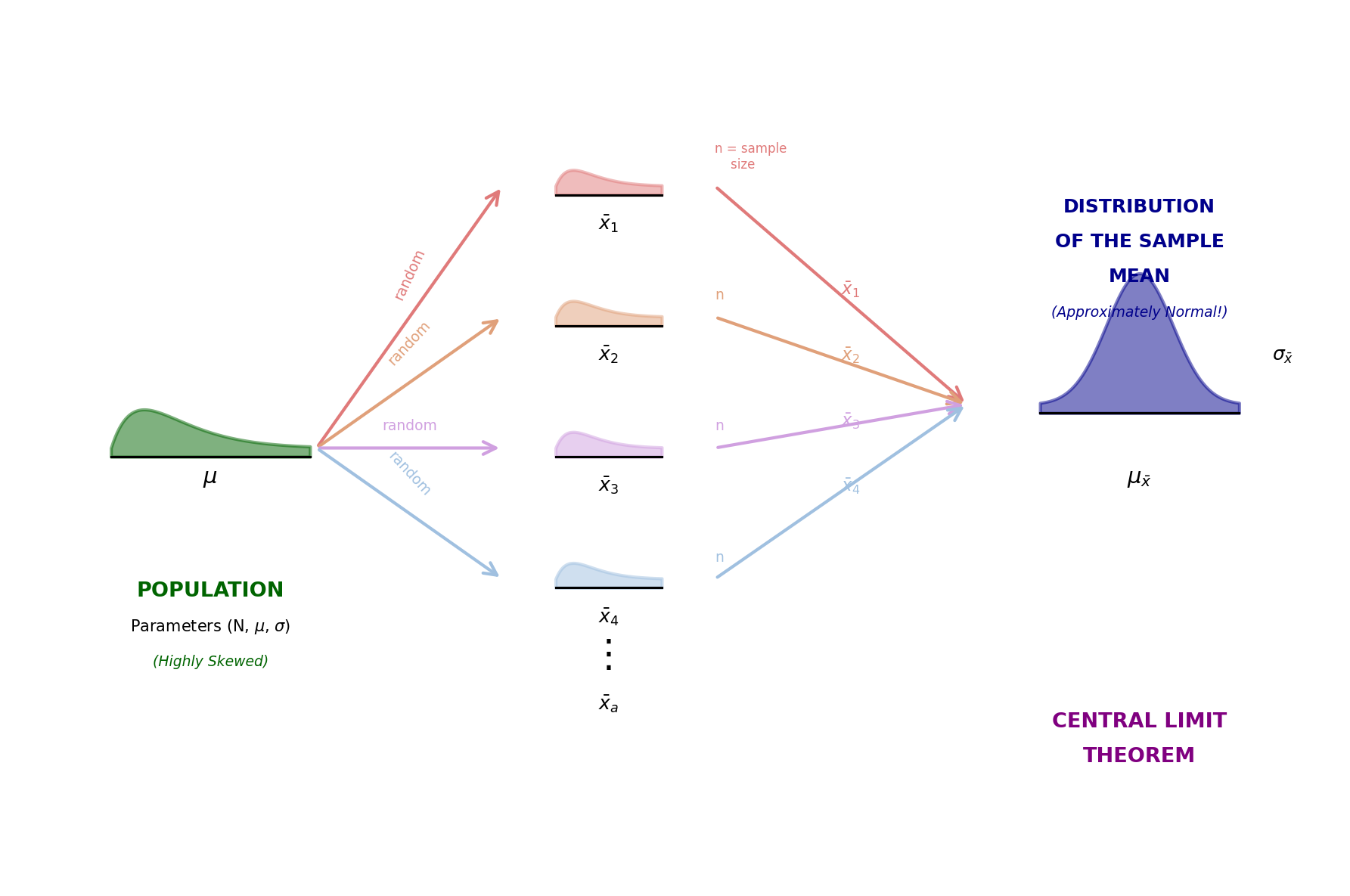
Sampling distribution of \(\bar{x}\)
(approximately normal!)
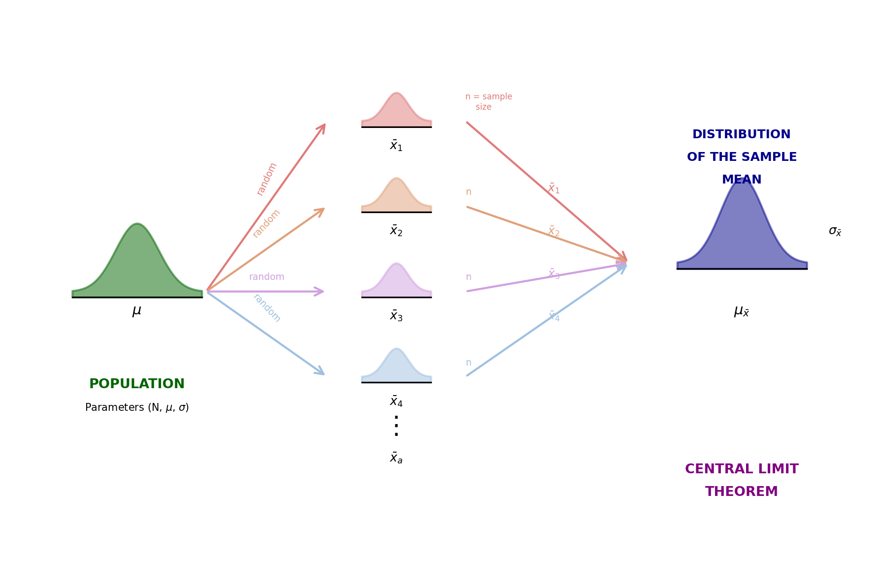
The magic: Regardless of the population’s shape, sample means follow a normal pattern!
Think-Pair-Share #3
Scenario: A biologist measures shell thickness in snails. The population distribution is heavily right-skewed (most snails have thin shells, few have very thick shells).
She takes samples of n = 40 snails at a time and calculates the average shell thickness for each sample.
Questions to discuss (2 minutes):
- Will the distribution of individual shell thicknesses be normal? Why or why not?
- Will the distribution of sample means (from many samples of 40) be approximately normal? Why?
- How does the CLT help us here?
Quick Report: What’s the difference between the population distribution and the sampling distribution? ✋
Standard Error
The standard error (SE) measures the typical distance between a sample statistic and the population parameter.
\[SE = \frac{\sigma}{\sqrt{n}}\]
Key insights:
- Larger samples (↑n) → smaller SE → more precise estimates
- More variable populations (↑σ) → larger SE → less precise estimates
From Sampling Distributions to Inference
Now we can connect these ideas to statistical inference:
- Point Estimates: Use \(\bar{x}\) to estimate μ
- Confidence Intervals: Create a range likely to contain μ
- Hypothesis Tests: Test claims about μ
All three rely on understanding sampling distributions!
Confidence Intervals: The Big Idea
- A point estimate (\(\bar{x}\) = 6.8 hours of sleep) is our best single guess
- But we know it varies from sample to sample (sampling variability!)
- A confidence interval creates a range that likely contains the true parameter
Example: “We are 95% confident that the average sleep duration of college students is between 6.5 and 7.1 hours”
What Does “95% Confident” Mean?
NOT: “There’s a 95% chance the true mean is in this interval”
YES: “If we repeated this process many times, about 95% of the intervals we create would contain the true population mean”
Analogy: It’s like a fishing net. We’re 95% confident our net caught the fish (parameter), but the fish is either in the net or not - there’s no probability to it once we’ve caught it.
Think-Pair-Share #4
Scenario: A health researcher wants to estimate the average daily water intake of adults. They survey 100 adults and calculate a 95% confidence interval: (1.8, 2.4) liters per day.
Questions to discuss (3 minutes):
- What does this interval tell us?
- Why is it a range rather than a single number?
- If they want a more precise estimate (narrower interval), what could they do?
- Does “95% confident” mean the true average is definitely in this interval?
Quick Report: How would you explain this confidence interval to someone without statistics training? ✋
Building Confidence Intervals
The general form:
\[\text{Point Estimate} \pm \text{Margin of Error}\]
For a population mean:
\[\bar{x} \pm z^* \times SE(\bar{x})\]
where:
- \(z^*\) is a critical value from a distribution (depends on confidence level, and choice of distribution depend on assumptions)
- \(SE(\bar{x}) = \frac{\sigma}{\sqrt{n}}\) is the standard error, that can be approximated by \(SE(\bar{x}) = \frac{s}{\sqrt{n}}\) when we don’t know \(\sigma\).
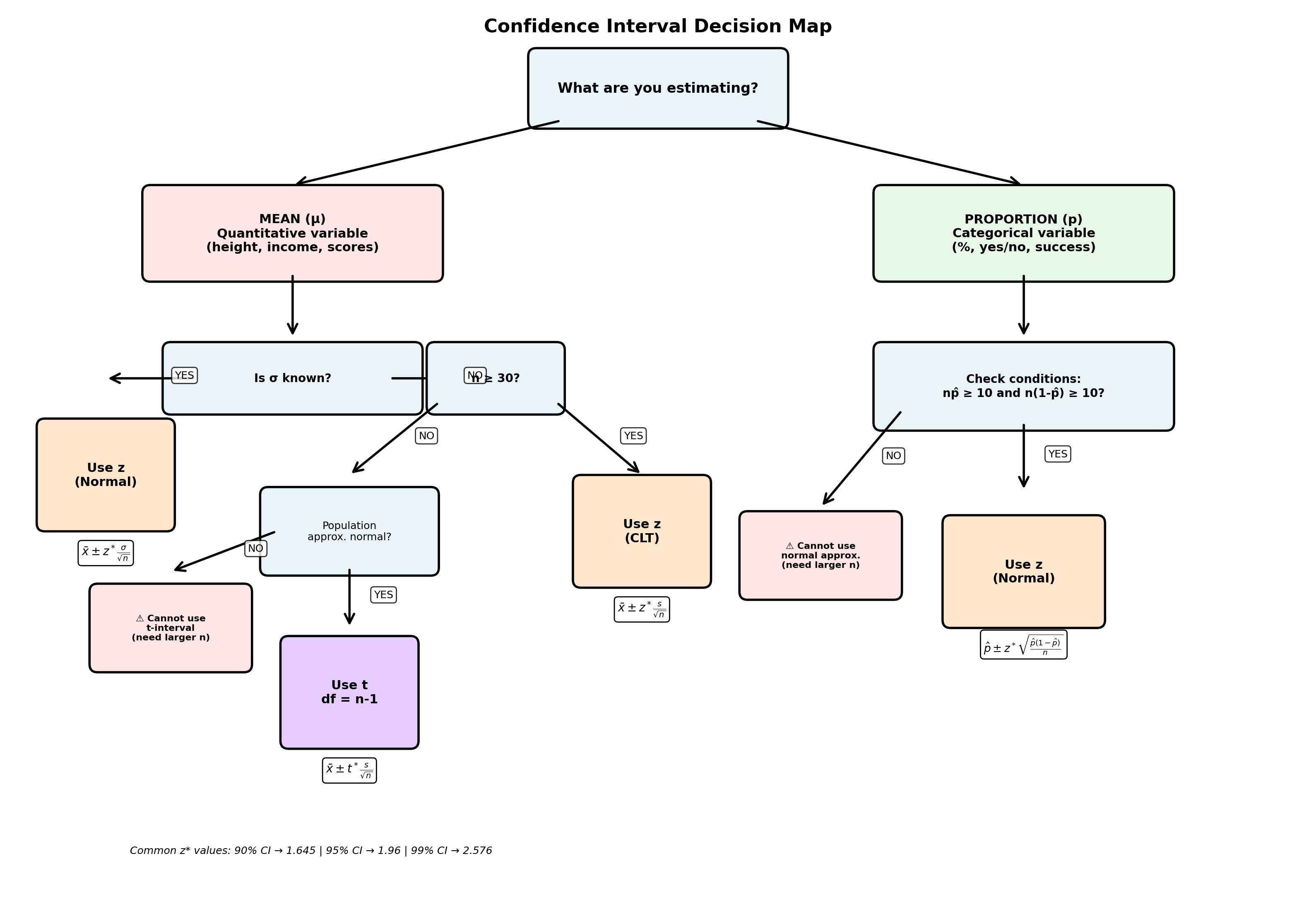
Confidence Intervals: Decision Map
First Question: What are you estimating?
Mean (μ)
Quantitative variable
(height, age, income, test scores)
Formula structure: \[\bar{x} \pm (\text{critical value}) \times SE\]
where \(SE = \frac{s}{\sqrt{n}}\)
Proportion (p)
Categorical variable
(% yes/no, success/failure)
Formula structure: \[\hat{p} \pm (\text{critical value}) \times SE\]
where \(SE = \sqrt{\frac{\hat{p}(1-\hat{p})}{n}}\)
Confidence Intervals for Means
Which distribution should you use?
Use Normal (z) ✓
Conditions: - Population \(\sigma\) is known, OR - Large sample (\(n \geq 30\)) AND \(\sigma\) unknown
Critical value: \(z^*\) from standard normal
(e.g., \(z^* = 1.96\) for 95% CI)
Formula: \[\bar{x} \pm z^* \frac{\sigma}{\sqrt{n}}\] or \[\bar{x} \pm z^* \frac{s}{\sqrt{n}}\]
Use t-distribution ✓
Conditions: - Population \(\sigma\) is unknown, AND - Small sample (\(n < 30\)), AND - Population is approximately normal
Critical value: \(t^*\) with \(df = n-1\)
(e.g., \(t^* \approx 2.09\) for 95% CI, \(n=20\))
Formula: \[\bar{x} \pm t^* \frac{s}{\sqrt{n}}\]
Note: Wider than z-interval (more uncertainty)
Confidence Intervals for Proportions
Use Normal (z) approximation
Conditions (must check!): 1. Random sample 2. \(n\hat{p} \geq 10\) 3. \(n(1-\hat{p}) \geq 10\)
Formula: \[\hat{p} \pm z^* \sqrt{\frac{\hat{p}(1-\hat{p})}{n}}\]
Common critical values: - 90% CI: \(z^* = 1.645\) - 95% CI: \(z^* = 1.96\) - 99% CI: \(z^* = 2.576\)
Example: In a survey of 200 students, 120 prefer online learning.
\(\hat{p} = 120/200 = 0.6\)
Check: \(200(0.6) = 120 \geq 10\) ✓ and \(200(0.4) = 80 \geq 10\) ✓
95% CI: \(0.6 \pm 1.96\sqrt{\frac{0.6(0.4)}{200}} = 0.6 \pm 0.068 = (0.532, 0.668)\)
What Affects Interval Width?
- Sample size (n): Larger n → narrower interval (more precise)
- Variability (s): More variable data → wider interval (less precise)
- Confidence level: Higher confidence (99% vs 95%) → wider interval (trade precision for confidence)
Key insight: There’s always a trade-off between precision and confidence!
Looking Ahead: Hypothesis Testing
Next class we’ll build on these ideas to test specific claims:
- “Is the average mercury level in fish above the safe threshold of 0.3 ppm?”
- “Do students sleep less than 8 hours on average?”
Preview: We’ll use sampling distributions to determine how likely we’d see our sample result if a claim were true.
Key Takeaways
- Statistics vary from sample to sample (sampling variability)
- Sampling distributions show the pattern of this variability
- Central Limit Theorem: Sample means are approximately normal for large enough n
- Standard error quantifies how much statistics typically vary
- Confidence intervals use these ideas to estimate parameters with uncertainty
Next Steps
- Next class: Hypothesis testing mechanics
- This week: DSA5 will give you hands-on practice with confidence intervals and t-tests in Google Sheets
- Preview the assignment so you know what we’re building toward!
Questions?