Lecture 8: Normal Distribution & Intro to Inference
STAT 7 - Statistical Methods for the Biological, Environmental & Health Sciences
10 Mar 2026
Welcome! Today’s Agenda
- Normal Distribution
- Normal Approximation to Binomial
- Sampling and Samples
- Parameters vs. Statistics
This is where probability meets inference!
Normal Distribution

The Normal Distribution
The most important continuous distribution in statistics!
Properties:
- Bell-shaped, symmetric curve
- Defined by two parameters: mean (\(\mu\)) and standard deviation (\(\sigma\))
- Notation: \(X \sim N(\mu, \sigma)\)
- Total area under curve = 1
- Many natural phenomena are approximately normal
Why Is It Called “Normal”?
History: The name comes from early statisticians who thought this distribution was the “norm” or typical pattern in nature.
Reality: It’s common but not universal!
- Heights, weights (within groups)
- Measurement errors
- Test scores (often designed to be)
- Averages of large samples (Central Limit Theorem!)
Normal Distribution Notation
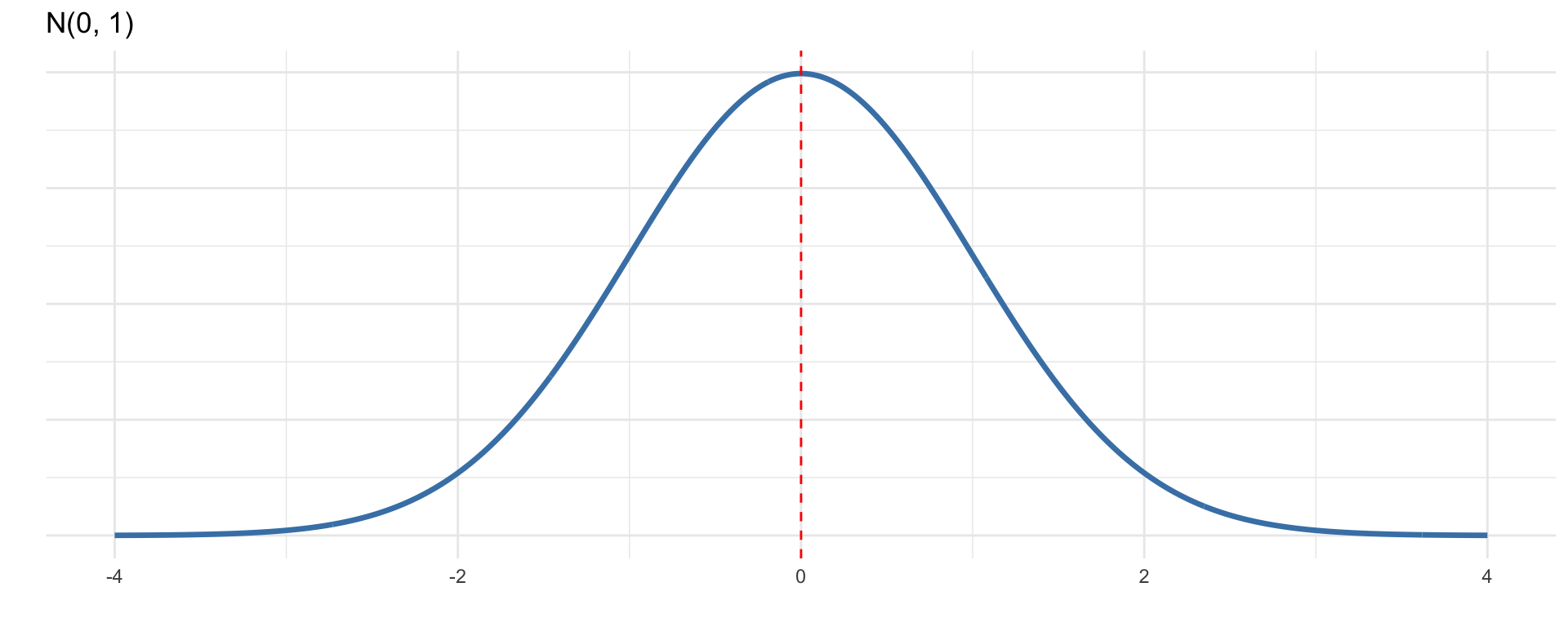
\[X \sim N(\mu, \sigma)\]
\(\mu = 0, \sigma = 1\)
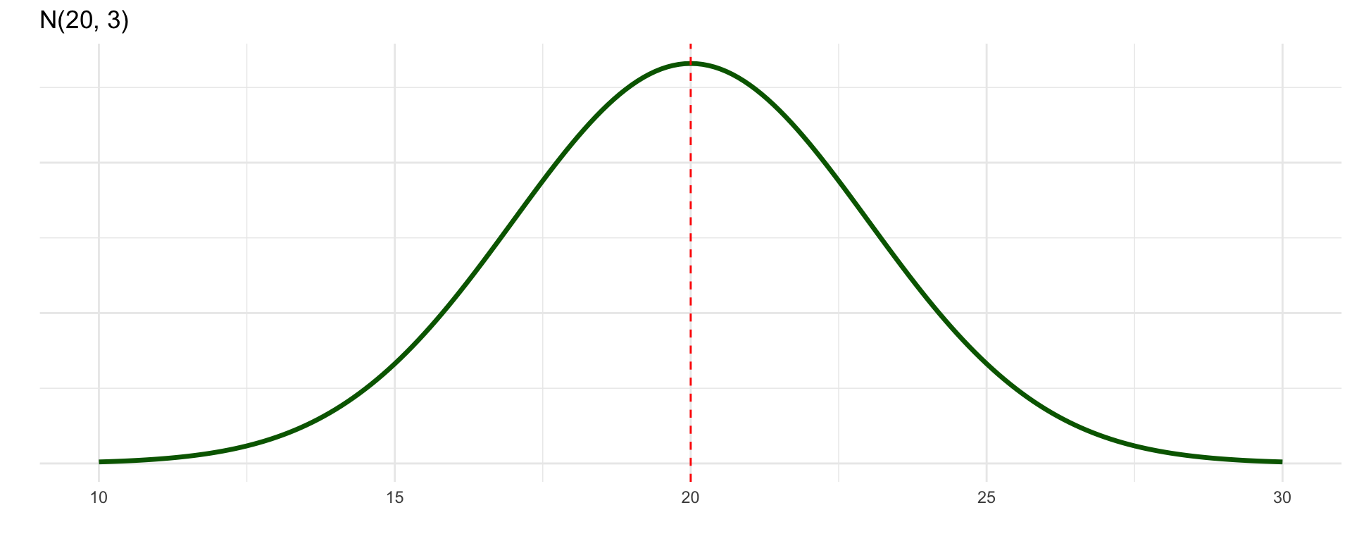
\(\mu = 20, \sigma = 3\)
Same shape, different location and spread!
The 68-95-99.7 Rule
Empirical Rule: For any normal distribution:
- 68% of data within 1 SD of mean
- 95% within 2 SD
- 99.7% within 3 SD
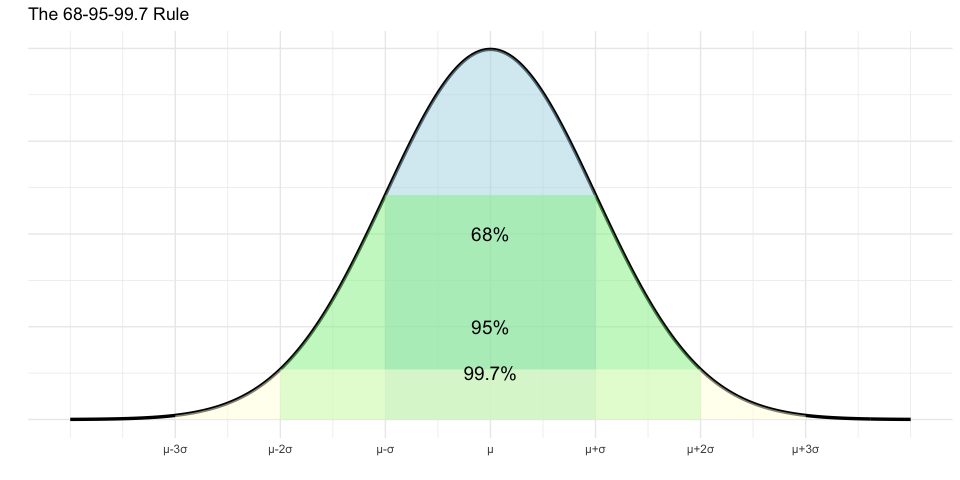
This is incredibly useful for quick estimates!
Example: Student Heights
Heights in this class are approximately \(N(168, 7)\) (cm)
Using the 68-95-99.7 rule:
- What percentage are between 161 and 175 cm?
- 161 = 168 - 7 and 175 = 168 + 7
- This is \(\mu \pm 1\sigma\), so ≈68%
- What percentage are between 154 and 182 cm?
- 154 = 168 - 14 and 182 = 168 + 14
- This is \(\mu \pm 2\sigma\), so ≈95%
- What percentage are taller than 168 cm?
- 168 = \(\mu\), and normal is symmetric
- 50%
Z-Scores: Standardizing
Z-score = number of standard deviations from the mean
\[z = \frac{x - \mu}{\sigma}\]
Properties:
- Positive z → above mean
- Negative z → below mean
- \(|z| > 2\) is “unusual”
Purpose: Allows comparison across different normal distributions!
Z-Score Example: Test Scores
SAT: \(N(1500, 300)\), ACT: \(N(21, 5)\)
- Pam scored 1800 on SAT
- Jim scored 24 on ACT
Who did better relative to their test?
Pam’s z-score: \[z = \frac{1800 - 1500}{300} = 1.0\]
Jim’s z-score: \[z = \frac{24 - 21}{5} = 0.6\]
Pam scored better (1 SD vs 0.6 SD above mean)
Using Google Sheets for Normal
NORM.DIST(x, mean, sd, cumulative)
- Returns P(X ≤ x) when cumulative = TRUE
- We almost always use cumulative = TRUE
NORM.INV(probability, mean, sd)
- Returns the x value with that cumulative probability
- Useful for finding percentiles
Example: For \(N(168, 7)\), what’s P(X ≤ 175)?
=NORM.DIST(175, 168, 7, TRUE) = 0.841
Practice: Normal Calculations
Heights: \(N(168, 7)\) cm
Calculate using Google Sheets:
- P(height > 168)
=1 - NORM.DIST(168, 168, 7, TRUE)= 0.50
- P(height between 161 and 175)
=NORM.DIST(175, 168, 7, TRUE) - NORM.DIST(161, 168, 7, TRUE)- = 0.841 - 0.159 = 0.682 ≈ 68%
- Find height of 70th percentile
=NORM.INV(0.70, 168, 7)= 171.7 cm
Interactive Demo
Let’s explore with the Normal Distribution App:
https://istats.shinyapps.io/NormalDist/
Try different values of \(\mu\) and \(\sigma\)!
Normal Distribution: More Examples
Example: Test scores are \(N(100, 15)\)
Using Google Sheets:
- What percentage have Test Score > 130?
=1 - NORM.DIST(130, 100, 15, TRUE)= 0.0228 ≈ 2.3%
- What Test Score score is the 90th percentile?
=NORM.INV(0.90, 100, 15)= 119.2
- What percentage have Test Score between 85 and 115?
=NORM.DIST(115, 100, 15, TRUE) - NORM.DIST(85, 100, 15, TRUE)- = 0.841 - 0.159 = 0.682 ≈ 68%
Checking for Normality
How do we know if data are approximately normal?
- Histogram - Is it roughly bell-shaped and symmetric?
- Q-Q Plot (Quantile-Quantile) - Do points fall on a straight line?
- 68-95-99.7 Rule - Does the data follow this pattern?
- Statistical tests - Shapiro-Wilk, Kolmogorov-Smirnov (later!)
Remember: Real data are never exactly normal, we look for “close enough”
Not Everything is Normal!
Examples of NON-normal distributions:
Right-skewed:
- Income
- House prices
- Time until failure
Left-skewed:
- Age at death (developed countries)
- Test scores (easy test)
Bimodal, uniform, etc.
Don’t force normality where it doesn’t exist!
Stretch Break!

Stand up, stretch, take a deep breath!
Normal Approximation to Binomial
Recall: Binomial Distribution
\(X \sim Bin(n, p)\) counts successes in n trials
- Discrete (whole numbers only)
- Can calculate exact probabilities
- But cumbersome for large n!
Question: Can we use the normal distribution to approximate?
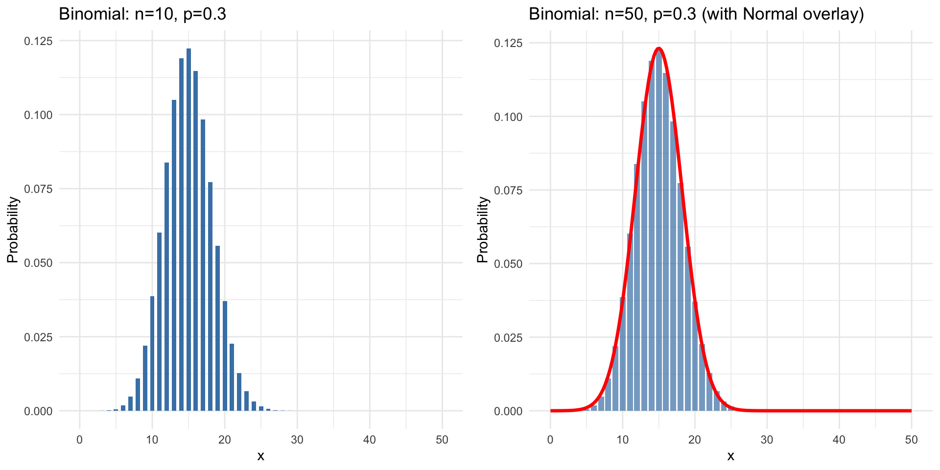
The Normal-Binomial Connection
When n is large, the binomial distribution starts to look normal!
When Can We Approximate?
Rule of thumb: Normal approximation is good when:
\[np \geq 10 \quad \text{AND} \quad n(1-p) \geq 10\]
Why these conditions?
- Ensures enough “successes” and “failures” expected
- Distribution is sufficiently symmetric
- Not too skewed to one side
If conditions met: Use \(N(\mu, \sigma)\) where:
\[\mu = np \qquad \sigma = \sqrt{np(1-p)}\]
Example: Should We Approximate?
Check if normal approximation is appropriate:
- n = 30, p = 0.5
- \(np = 30(0.5) = 15 \geq 10\) ✓
- \(n(1-p) = 30(0.5) = 15 \geq 10\) ✓
- YES, use approximation
- n = 100, p = 0.05
- \(np = 100(0.05) = 5 < 10\) ✗
- NO, don’t use approximation
- n = 500, p = 0.03
- \(np = 500(0.03) = 15 \geq 10\) ✓
- \(n(1-p) = 500(0.97) = 485 \geq 10\) ✓
- YES, use approximation
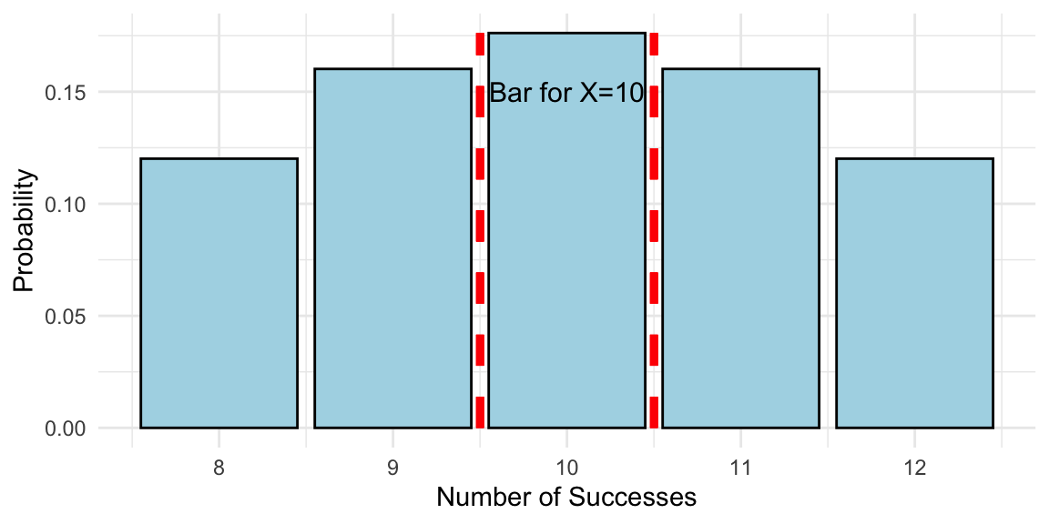
Continuity Correction
Problem: Binomial is discrete, Normal is continuous
Solution: Continuity correction
- For P(X ≤ k), use P(X < k + 0.5)
- For P(X ≥ k), use P(X > k - 0.5)
- For P(X = k), use P(k - 0.5 < X < k + 0.5)
Why? The bar for X = k extends from k - 0.5 to k + 0.5
Example: Normal Approximation
Setup: Flip a fair coin 100 times. Find P(X ≥ 60) where X = # heads.
Check conditions:
- \(np = 100(0.5) = 50 \geq 10\) ✓
- \(n(1-p) = 100(0.5) = 50 \geq 10\) ✓
Using normal approximation:
\[\mu = np = 50, \quad \sigma = \sqrt{np(1-p)} = \sqrt{25} = 5\]
With continuity correction: P(X ≥ 60) ≈ P(Z > 59.5)
In Google Sheets: =1 - NORM.DIST(59.5, 50, 5, TRUE) = 0.0287
About 2.9% chance of 60+ heads
Comparison: Exact vs Approximate
For the coin example (n=100, p=0.5):
Exact (using Binomial):
=1 - BINOM.DIST(59, 100, 0.5, TRUE)Result: 0.0284
Approximate (using Normal):
=1 - NORM.DIST(59.5, 50, 5, TRUE)Result: 0.0287
Very close! Normal approximation works well here.
From Probability to Inference
The Big Picture
So far (Weeks 1-4):
- Described data
- Calculated probabilities
- Modeled random variables
Descriptive statistics & Probability
Coming up (Weeks 5-10):
- Make inferences about populations
- Test hypotheses
- Estimate parameters
Inferential statistics
Bridge: Sampling distributions!
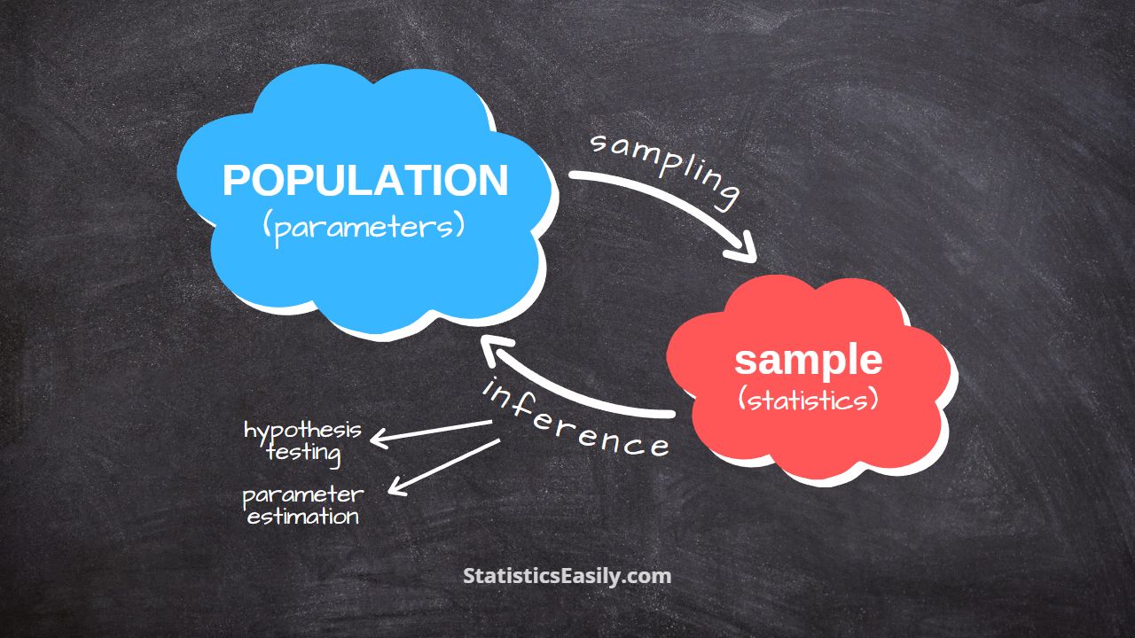
Populations vs Samples
Population
- All individuals of interest
- Usually large or infinite
- Parameters describe it
- Often unknown
Examples:
- μ (population mean)
- σ (population SD)
- p (population proportion)
Sample
- Subset of population
- Practical to collect
- Statistics describe it
- We calculate these
Examples:
- \(\bar{x}\) (sample mean)
- s (sample SD)
- \(\hat{p}\) (sample proportion)
Parameters vs Statistics
Key distinction:
Parameter → Population → Unknown (usually)
Statistic → Sample → Known (calculated)
Goal of inference: Use statistics to estimate parameters!
Example: Parameters vs Statistics
Scenario: Study average sleep hours of UCSC students
- Population: All UCSC students Winter 2026 (~20,000)
- Parameter of interest: μ = true average sleep hours
- Sample: 100 randomly selected students
- Statistic: \(\bar{x}\) = 6.8 hours (from our sample)
Question: Is \(\bar{x} = 6.8\) exactly equal to μ?
Answer: Probably not! There’s sampling variability
Sampling Variability
Key insight: Different samples give different statistics!
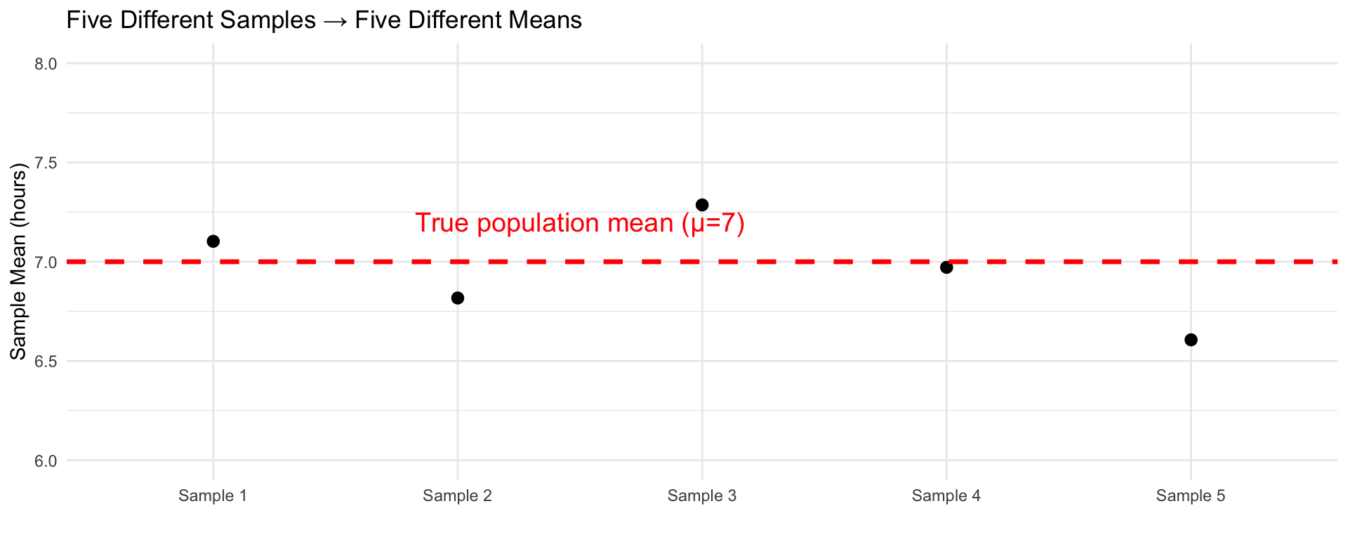
This is natural and expected!
The Path Forward
What we’ve built:
- Probability foundations ✓
- Random variables & distributions ✓
- Sampling distributions ✓
What’s next (Week 5+):
- Review for the midterm (Tuesday) come with questions!
- Thursday: midterm
- Week 6: Sampling Distributions and Central Limit Theorem
Exit Ticket
Before you leave:
- Post the solutions to these on Ed Discussion:
Name one new thing you learned today
Check approximation: n=50, p=0.15. Can we use normal approximation?
- Due Friday:
- HW 3
- Complete during DS:
- DSA 3
Questions?
Office hours: I’ll be in the classroom nextdoor after class if you need me. If you can’t stay, check our office hours on Ed Discussion and look for a spot that works with your schedule.
Practice is essential: Don’t forget to think deeply when solving your assignments. Don’t do it as a check list, but rather as an opportunity to think about the concepts that we have learned.
Have a nice weekend!
See you next week!
Sampling Distributions
What is a Sampling Distribution?
Definition: The probability distribution of a statistic across all possible samples of size n
- Not the distribution of the data
- Distribution of the statistic (e.g., \(\bar{x}\))
- Shows how the statistic varies from sample to sample
- Theoretical concept (we imagine all possible samples)
Building Intuition
Thought experiment:
- Take a random sample of n=30 students, calculate \(\bar{x}\)
- Take another sample of n=30, calculate \(\bar{x}\) again
- Repeat thousands of times
- Make a histogram of all the \(\bar{x}\) values
That histogram approximates the sampling distribution of \(\bar{x}\)
Sampling Distribution Simulation
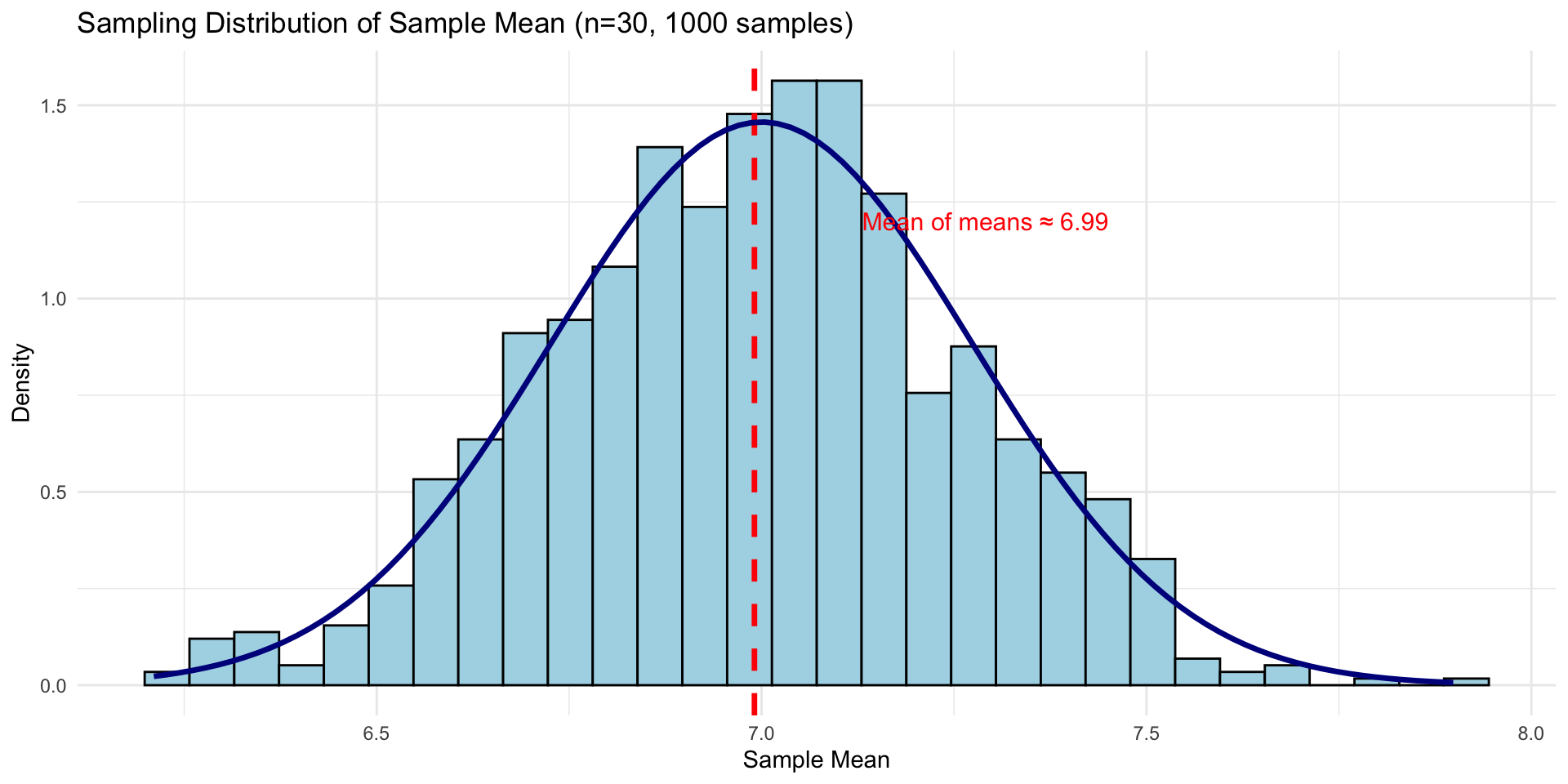
Notice: It’s approximately normal and centered at μ!
Properties of Sampling Distribution of \(\bar{x}\)
For samples of size n from a population with mean μ and SD σ:
1. Center: \[E(\bar{x}) = \mu\]
The mean of the sampling distribution equals the population mean
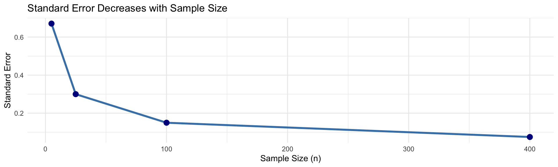
2. Spread: \[SD(\bar{x}) = \frac{\sigma}{\sqrt{n}}\]
Called the standard error (SE)
3. Shape: Depends on population and sample size (more soon!)
Standard Error vs Standard Deviation
Important distinction!
Standard Deviation (σ)
- Measures spread of individuals in population
- Does NOT depend on sample size
- Describes population variability
Standard Error (SE)
- Measures spread of sample means
- \(SE = \frac{\sigma}{\sqrt{n}}\)
- Decreases as n increases
- Describes sampling variability
Why Does SE Decrease with n?
\[SE = \frac{\sigma}{\sqrt{n}}\]
Intuition: Larger samples give more stable estimates
- Sample of n=1: Very unreliable, high variability
- Sample of n=100: Much more reliable, low variability
- Sample of n=10,000: Very reliable, very low variability
The Central Limit Theorem (CLT)
One of the most important theorems in statistics!
Central Limit Theorem Statement
For samples of size n from ANY population with mean μ and SD σ:
As n increases, the sampling distribution of \(\bar{x}\) becomes approximately normal with:
- Mean = μ
- Standard deviation = \(\frac{\sigma}{\sqrt{n}}\)
In notation:
\[\bar{x} \sim N\left(\mu, \frac{\sigma}{\sqrt{n}}\right) \quad \text{approximately, for large } n\]
What Makes CLT Amazing?
- Works for ANY population distribution (skewed, bimodal, anything!)
- Only needs n to be “large enough” (usually n ≥ 30)
- Explains why normal distribution is so common
- Foundation for most inferential statistics
CLT Visualization
Original population: Right-skewed (NOT normal)
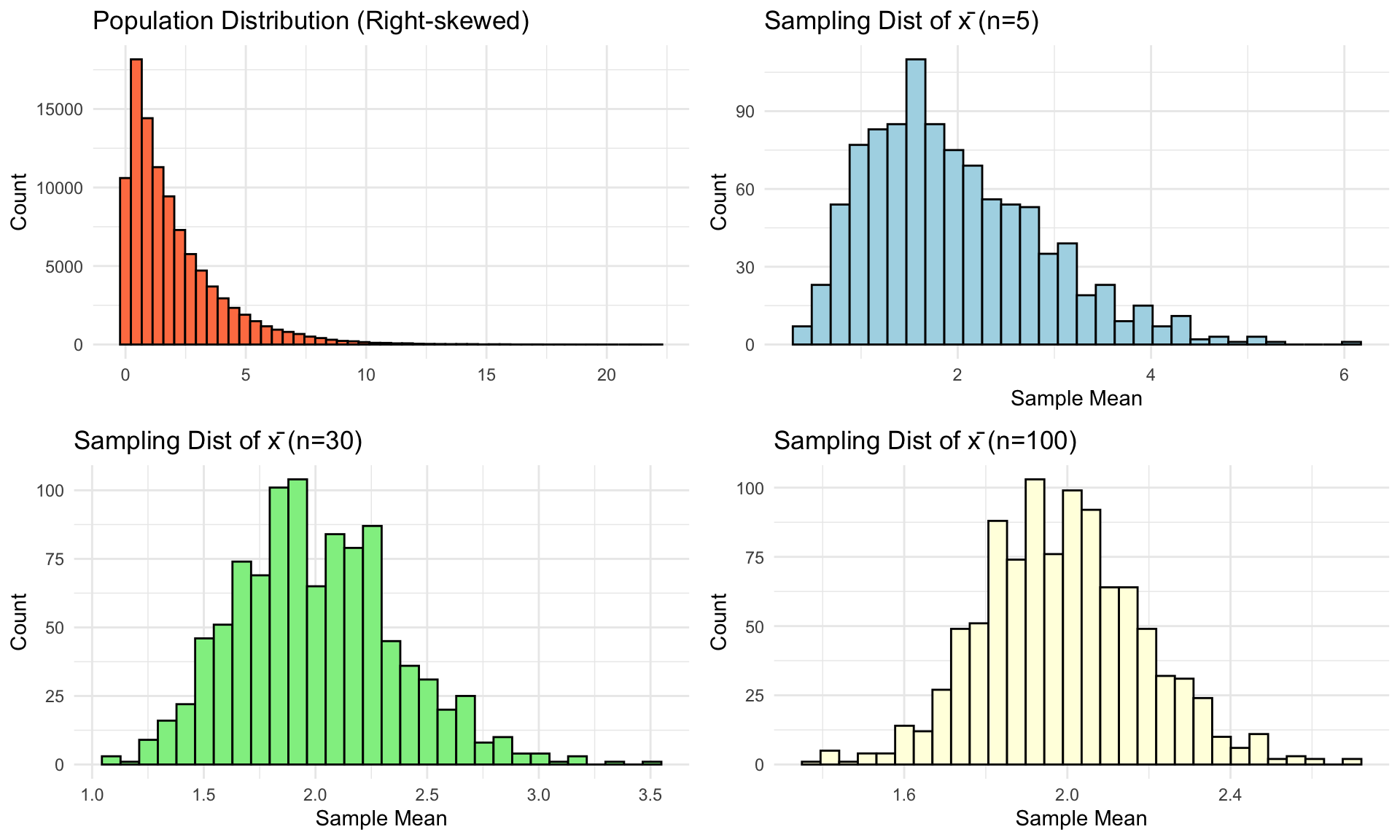
Notice: As n increases, sampling distribution becomes normal!
When Does CLT Apply?
General rule: n ≥ 30 is usually sufficient
BUT this depends on population shape:
- Population is normal: CLT applies for ANY n (even n=1!)
- Population is symmetric: n ≥ 15 usually fine
- Population is moderately skewed: n ≥ 30 needed
- Population is heavily skewed: May need n ≥ 50 or more
Key point: More skewed population → need larger n
Example: Using the CLT
Problem: Average adult height μ = 170 cm, σ = 10 cm.
For a random sample of n = 36 adults, find P(\(\bar{x}\) > 172).
Solution:
By CLT, \(\bar{x} \sim N(170, \frac{10}{\sqrt{36}}) = N(170, 1.67)\)
In Google Sheets:
=1 - NORM.DIST(172, 170, 1.67, TRUE)Result: 0.115
About 11.5% chance the sample mean exceeds 172 cm
CLT Application: Quality Control
Scenario: Light bulb manufacturer
- Population: μ = 1000 hours, σ = 100 hours
- Take sample of n = 25 bulbs
- Want P(990 < \(\bar{x}\) < 1010)
Solution:
\(\bar{x} \sim N(1000, \frac{100}{\sqrt{25}}) = N(1000, 20)\)
=NORM.DIST(1010, 1000, 20, TRUE) - NORM.DIST(990, 1000, 20, TRUE)Result: 0.383
38.3% of samples will have mean between 990-1010 hours
Summary: Key Distributions
| Distribution | Type | When to Use | Parameters |
|---|---|---|---|
| Binomial | Discrete | Count successes in n trials | n, p |
| Normal | Continuous | Symmetric, bell-shaped data | μ, σ |
| Sampling Dist of \(\bar{x}\) | Theoretical | Distribution of sample means | μ, σ/√n |
Remember: CLT tells us the third one is approximately Normal!
Common Misconceptions
- “CLT makes the population distribution normal”
- NO! It makes the sampling distribution of \(\bar{x}\) normal
- “Larger samples reduce bias”
- NO! They reduce variability (SE decreases)
- Bias is a systematic error, not fixed by sample size
- “Standard error and standard deviation are the same”
- NO! SD measures individual variability, SE measures sampling variability
- “Normal approximation always works for binomial”
- NO! Only when np ≥ 10 AND n(1-p) ≥ 10
Summary:
- Normal approximation to binomial (when np ≥ 10 and n(1-p) ≥ 10)
- Parameters (population) vs Statistics (sample)
- Sampling distributions show how statistics vary
- Standard Error = SD of sampling distribution = σ/√n
- Central Limit Theorem: Sampling distribution of \(\bar{x}\) is approximately N(μ, σ/√n) for large enough n
This is the foundation for all of inferential statistics!
![]()
STAT 7 – Winter 2026