Lecture 5: Probability Foundations & Conditional Probability

STAT 7 - Statistical Methods for the Biological, Environmental & Health Sciences

Prof. Marcela Alfaro Córdoba

Statistics - UCSC

10 Mar 2026

Welcome! Quick Check-in

Poll Time!

PollEv.com/slugstats

How confident do you feel about the probability concepts we’ve started exploring?

• Very confident
• Somewhat confident
  
• Not very confident
• What’s this class about?

Week at a Glance

Day	Topics	To-Do
Tuesday	Probability foundations, conditional probability	Attend lecture, participate in activities
Thursday	Bayes’ Theorem, diagnostic testing	Attend lecture, participate in activities
Friday	-	HW2 due
Discussion	Practice with EDA	DSA 3 due after section, Section C is due before class on Thursday

Part 1: Motivation

HIV Testing & Public Health

Case Study: HIV Screening

The Scenario:

A 23-year-old patient gets tested for HIV at a community health clinic. The test comes back positive.

Questions to Consider:

• What’s the probability they actually have HIV?
• Does a positive test mean they definitely have the disease?
• What other information do we need?

HIV Test Kit

The Numbers

According to the CDC (2024 estimates):

• Prevalence of HIV in young adults (18-24): ~0.2%
• Test sensitivity (true positive rate): 99.7%
• Test specificity (true negative rate): 98.5%

Think about this:
If we test 10,000 people, what happens?

Think-Pair-Share

Your Task

Individual Think (2 min):

Imagine we test 10,000 people. Given:

• 0.2% have HIV
• Test is 99.7% sensitive
• Test is 98.5% specific

How many people would test positive? How many of those actually have HIV?

Pair Discussion (3 min): Share your thinking with a neighbor

Share Out: Let’s hear some approaches!

Building Our Tools

To answer this question properly, we need to understand:

1. Probability foundations - sample spaces, events, rules
2. Probability distributions - organizing outcomes
3. Conditional probability - P(has HIV | tested positive)
4. Tree diagrams - organizing sequential events
5. Contingency tables - displaying joint probabilities

Let’s build these tools step by step.

Part 2: Probability Review

Core concepts and rules

Why Probability?

To understand statistical inference, we need probability!

Random Phenomena

Definition

We know what outcomes could happen, but we don’t know which particular values will be observed.

Examples:

• Rolling dice 🎲
• Coin flips 🪙
• Drawing cards 🃏
• Selecting random samples
• Medical test results

Basic Probability Concepts

• Random phenomenon: Outcomes we cannot predict with certainty, but that have a regular distribution in many repetitions

• Probability: The proportion of times an outcome occurs in many repeated trials

• Independent trials: The outcome of one trial does not influence another

Sample Space and Events

Sample Space (S): Set of all distinct possible outcomes

• Example (rolling a die): S = {1, 2, 3, 4, 5, 6}

Event: An outcome or set of outcomes (subset of sample space)

• Example: A = “rolling an even number” = {2, 4, 6}

Probability of an event: P(A) = |A| / |S| = 3/6 = 1/2

Probability Rules

Three Key Properties

1. Each probability must be between 0 and 1
2. All probabilities must sum to 1
3. The probability of any event is the sum of the probabilities of its outcomes

Addition Rule: Disjoint Events

If A₁ and A₂ are disjoint (mutually exclusive):

\[P(A_1 \text{ or } A_2) = P(A_1) + P(A_2)\]

Example: Rolling a die

• A = {2, 4, 6} (even numbers)
• B = {1, 3, 5} (odd numbers)
• P(A or B) = P(A) + P(B) = 1/2 + 1/2 = 1

General Addition Rule

For any two events A and B:

\[P(A \text{ or } B) = P(A) + P(B) - P(A \text{ and } B)\]

Example: Rolling a die

• A = {2, 4, 6}
• B = {1, 2, 3, 5}
• P(A or B) = 3/6 + 4/6 - 1/6 = 6/6 = 1

Complement Rule

The complement of event A is Aᶜ:

\[P(A) + P(A^c) = 1\]

Therefore: \[P(A) = 1 - P(A^c)\]

Example: Rolling a die

• P(not getting 1) = 1 - P(getting 1) = 1 - 1/6 = 5/6

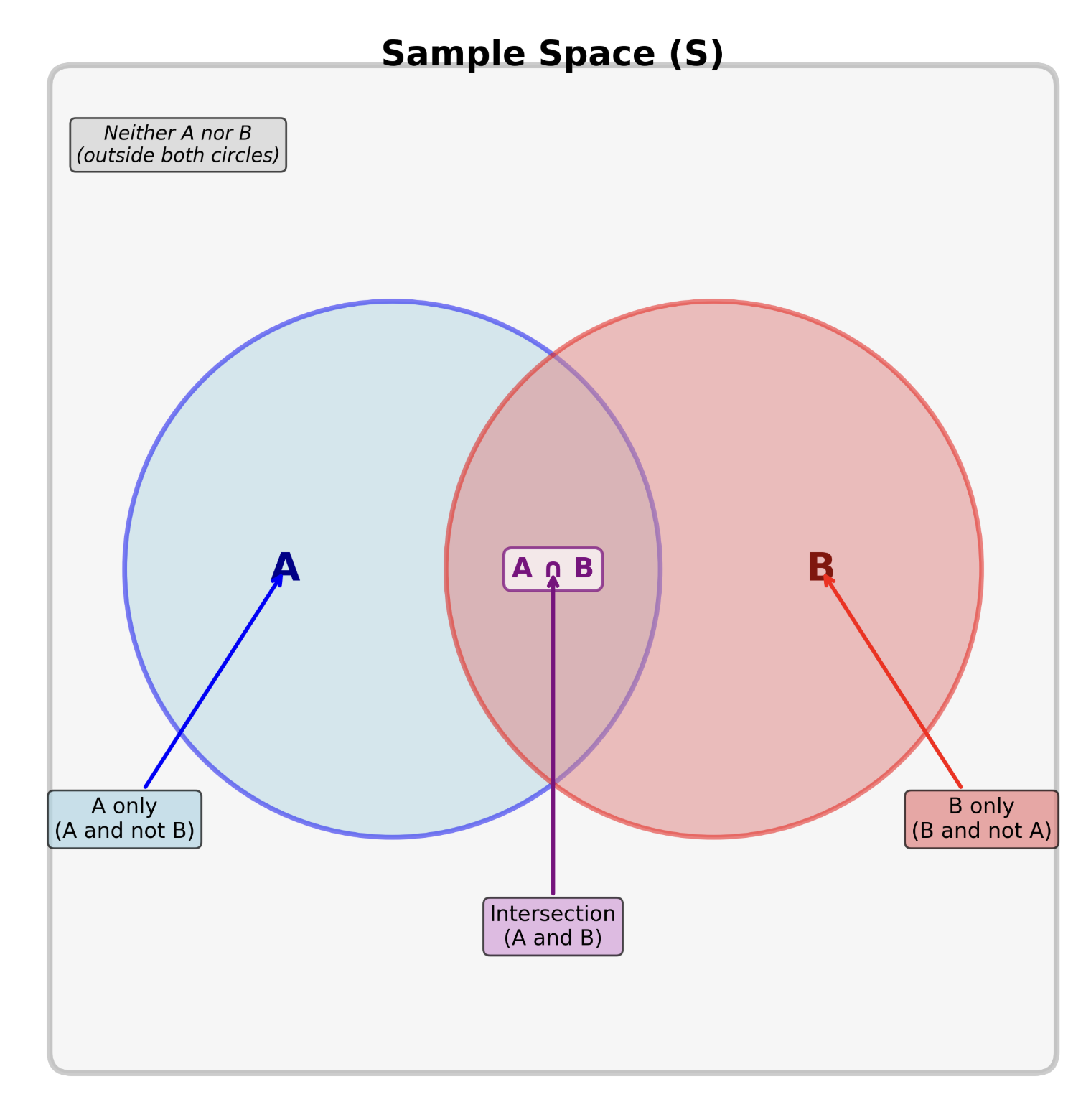
Activity: Venn Diagram Identification

Your Task

Venn diagram showing sample space, event D and complement

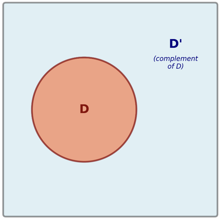
Mark all the events present:

• Sample Space (S)
• Event D and Dᶜ
• Disjoint Events
• Complement events

Multiplication Rule: Independent Events

If A and B are independent:

\[P(A \text{ and } B) = P(A) \times P(B)\]

Warning

Important: Do not confuse disjoint and independent!

• Disjoint: Cannot happen together (P(A and B) = 0)
• Independent: One doesn’t affect the other

Independence Example

Two dice illustration

Rolling two dice:

• First die shows 1: probability = 1/6
• Second die shows 1: probability = 1/6
• Both show 1: P = (1/6) × (1/6) = 1/36

The first roll doesn’t affect the second!

Part 3: Probability Distributions

Organizing outcomes and probabilities

Probability Distribution

Definition

A probability distribution lists all possible outcomes and their associated probabilities, satisfying:

1. Outcomes must be disjoint
2. Each probability must be between 0 and 1
3. Probabilities must total to 1

Activity: Patient Satisfaction

Hospital Survey Data

	Very satisfied	Somewhat satisfied	Neither	Somewhat dissatisfied	Very dissatisfied
Probability	0.32	0.35	0.13	0.07	0.13

Questions: 1. Can this be a probability distribution? 2. What is P(satisfied or very satisfied)?

Poll: PollEv.com/slugstats

Solution: Patient Satisfaction

Question 1: Can this be a probability distribution?

Check the three rules:

1. ✓ Outcomes are disjoint (can’t be both “very satisfied” and “somewhat dissatisfied”)
2. ✓ Each probability is between 0 and 1
3. ✓ Sum: 0.32 + 0.35 + 0.13 + 0.07 + 0.13 = 1.00

Yes, this is a valid probability distribution!

Solution: Patient Satisfaction (cont.)

Question 2: P(satisfied or very satisfied)?

Since these events are disjoint, we can add:

P(somewhat satisfied or very satisfied) = P(somewhat) + P(very)

= 0.35 + 0.32 = 0.67

Interpretation: 67% of patients report being satisfied or very satisfied.

Activity: Practice Problems

Rolling One Die

S = {1, 2, 3, 4, 5, 6}, A = {1, 2, 3}, B = {2, 3, 4, 5, 6}

Calculate:

1. P(A ∩ B) = ?
2. P(A ∪ B) = P(A) + P(B) - P(A ∩ B) = ?
3. P(Bᶜ) = 1 - P(B) = ?

Poll: PollEv.com/slugstats

Solution: Die Rolling Practice

Given: S = {1, 2, 3, 4, 5, 6}, A = {1, 2, 3}, B = {2, 3, 4, 5, 6}

1. P(A ∩ B) = P(A and B) = P({2, 3}) = 2/6 = 1/3

2. P(A ∪ B) = P(A) + P(B) - P(A ∩ B) = 3/6 + 5/6 - 2/6 = 6/6 = 1

3. P(Bᶜ) = 1 - P(B) = 1 - 5/6 = 1/6

   (Note: Bᶜ = {1}, so P(Bᶜ) = 1/6 ✓)

Break Time! ☕ 5-minute break

Stretch, grab water, chat with neighbors!

We’ll resume with conditional probability.

Part 4: Conditional Probability

When prior information changes what we know

Marginal and Joint Probability

Let’s look at data on diabetes and age from a large health survey:

	Diabetes	No Diabetes	Total
Less than 20 years	0.001	0.277	0.277
20 to 44 years	0.014	0.315	0.329
45 to 64 years	0.043	0.219	0.261
Greater than 64	0.036	0.097	0.132
Total	0.093	0.907	1.000

Reading the Table

	Diabetes	No Diabetes	Total
Less than 20 years	0.001	0.277	0.277
20 to 44 years	0.014	0.315	0.329
45 to 64 years	0.043	0.219	0.261
Greater than 64	0.036	0.097	0.132
Total	0.093	0.907	1.000

• Joint probabilities: Interior cells (e.g., 0.043)
• Marginal probabilities: Row and column totals (e.g., 0.093, 0.261)

Is this a Probability Distribution?

Check the Rules

How can we verify this is a valid joint probability distribution?

1. Are the outcomes disjoint?
2. Are all probabilities between 0 and 1?
3. Do they sum to 1?

Think for 30 seconds, then we’ll discuss!

Verification

1. Disjoint outcomes? ✓
Each person falls into exactly one cell (e.g., can’t be both “20-44” and “45-64”)

2. Between 0 and 1? ✓
All values are probabilities: 0.001, 0.014, …, 0.907

3. Sum to 1? ✓
All interior cells: 0.001 + 0.277 + 0.014 + … = 1.000

Yes! This is a valid probability distribution.

What is Conditional Probability?

Conditional Probability is the probability of an event occurring, given that another event has already occurred.

Notation: P(A | B)
Read as: “Probability of A given B”

Example from daily life:

• P(traffic jam | rush hour)
• P(rain | cloudy sky)
• P(passing exam | studied)

Biological examples:

• P(disease | positive test)
• P(recovery | treatment)
• P(mutation | exposure)

Visual Intuition

Venn diagram showing events A and B in sample space S

Unconditional: P(A)
All of A divided by all of S

Venn diagram with focus on region B, showing A∩B within B

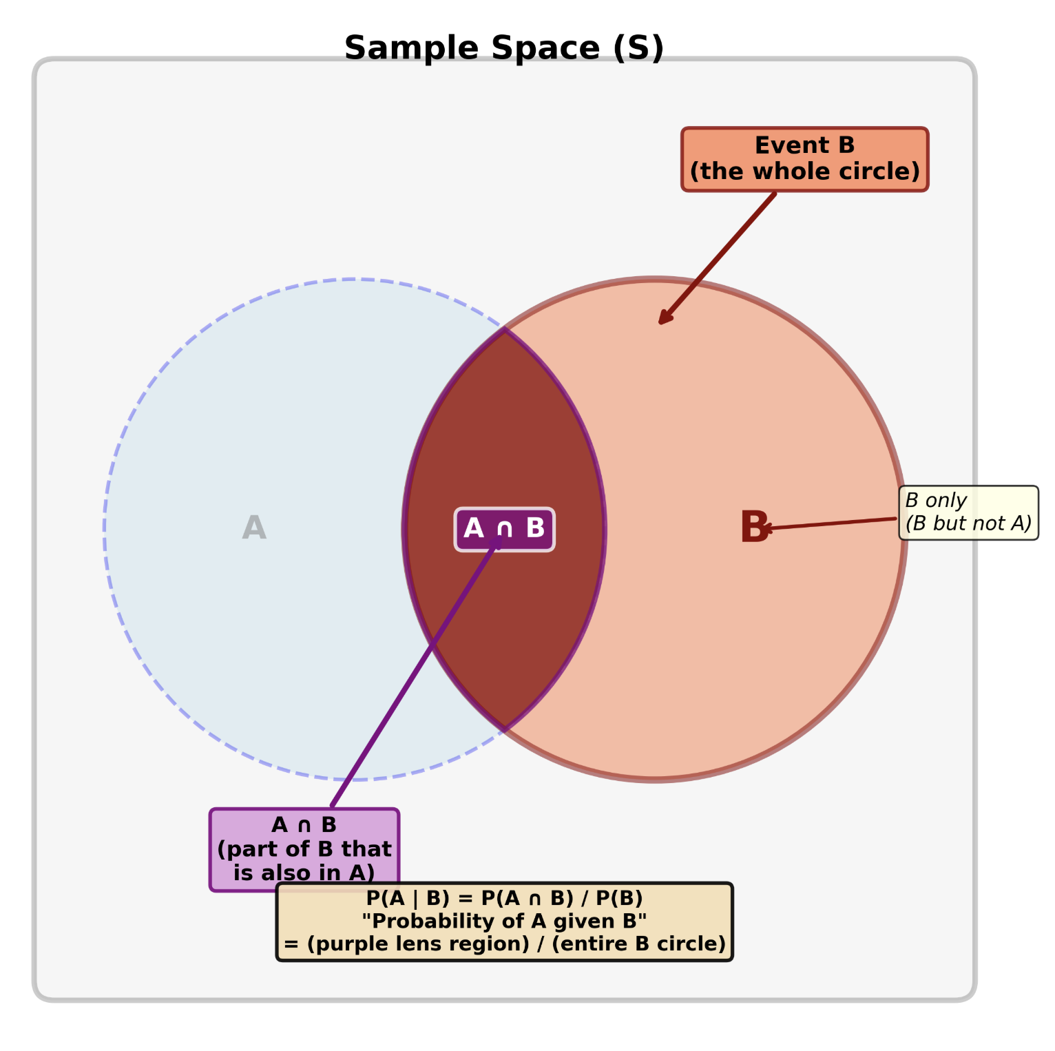
Conditional: P(A | B)
A and B divided by B
We’ve restricted our sample space!

The Formula

Conditional Probability Formula

\[P(A|B) = \frac{P(A \text{ and } B)}{P(B)}\]

provided that P(B) > 0

Intuition:

• We’re “zooming in” on only the outcomes where B occurred
• Among those, what fraction also has A?

Example: Diabetes & Age

Using our diabetes table:

	Diabetes	No Diabetes	Total
45 to 64 years	0.043	0.219	0.261

Question: What’s the probability someone has diabetes, given they’re 45-64 years old?

\[P(\text{Diabetes | Age 45-64}) = \frac{P(\text{Diabetes and Age 45-64})}{P(\text{Age 45-64})}\]

Calculating P(Diabetes | Age 45-64)

\[P(\text{Diabetes | Age 45-64}) = \frac{P(\text{Diabetes and Age 45-64})}{P(\text{Age 45-64})}\]

From the table:

• P(Diabetes and Age 45-64) = 0.043
• P(Age 45-64) = 0.261

Calculate: \[P(\text{Diabetes | Age 45-64}) = \frac{0.043}{0.261}\] \[= 0.1647 \approx 16.5\%\]

Interpretation: Among people aged 45-64, about 16.5% have diabetes.

Compare: Unconditional vs. Conditional

Unconditional probability:

P(Diabetes) = 0.093 = 9.3%

In the general population

Conditional probability:

P(Diabetes | Age 45-64) = 0.1647 = 16.5%

Among 45-64 year olds

Why the difference?
Age gives us information! Being in the 45-64 age group increases the probability of having diabetes compared to the general population.

Activity: Your Turn!

Calculate and Compare

Using the same diabetes table:

Question: What’s P(Age 45-64 | Diabetes)?

Individual (2 min): Set up and solve

Pair (3 min):

• Compare answers
• Discuss: Is this the same as P(Diabetes | Age 45-64)? Why or why not?

Poll: PollEv.com/slugstats

Solution: P(Age 45-64 | Diabetes)

\[P(\text{Age 45-64 | Diabetes}) = \frac{P(\text{Age 45-64 and Diabetes})}{P(\text{Diabetes})}\]

Calculate: \[= \frac{0.043}{0.093} = 0.4624 \approx 46.2\%\]

Interpretation: Among people with diabetes, about 46.2% are in the 45-64 age group.

Important

Remember: P(A|B) ≠ P(B|A) in general!

The order matters in conditional probability!

Independence Revisited

Recall: Events A and B are independent if
P(A and B) = P(A) × P(B)

New perspective with conditional probability:

Independence Definition

A and B are independent if and only if:

\[P(A|B) = P(A)\]

or equivalently:

\[P(B|A) = P(B)\]

Meaning: Knowing B occurred doesn’t change the probability of A

Example: Testing Independence

Are “having diabetes” and “being age 45-64” independent?

Check if P(Diabetes | Age 45-64) = P(Diabetes):

• P(Diabetes | Age 45-64) = 0.1647 ≈ 16.5%
• P(Diabetes) = 0.093 = 9.3%

Since 16.5% ≠ 9.3%, these events are NOT independent.

Knowing someone’s age group gives us information about their diabetes status!

Wrapping Up

Key takeaways from today

Today’s Key Concepts

1. Probability foundations: Sample space, events, rules

   • Addition rule, complement rule, multiplication rule

2. Probability distributions: Valid when outcomes are disjoint, probabilities sum to 1

3. Conditional Probability: P(A|B) = P(A and B) / P(B)

   • Order matters! P(A|B) ≠ P(B|A) in general

4. Independence: P(A|B) = P(A) when A and B are independent

5. Tree Diagrams & Tables: Two ways to organize the same information

Quick Knowledge Check

Poll Time!

PollEv.com/slugstats

Question: If P(A) = 0.3, P(B) = 0.4, and P(A and B) = 0.12, are A and B independent?

A. Yes
B. No
C. Need more information

Questions?

Post on Ed Discussion or come to office hours!

Office Hours:
I’ll be here after class :)

Next class: Thursday, January 23rd
Bayes’ Theorem & Diagnostic Testing

See you then! 🦠🔬📊