🗓️ Week 09
Regularized Regression

STAT 204 – Introduction to Statistical Data Analysis

Prof. Marcela Alfaro Cordoba

Statistics - UCSC

25 Nov 2025

Linear Regression Review

\[Y_i = \beta_0 + \beta_1X_{i1} + \cdots + \beta_pX_{ip} + \epsilon_i\]

\[\widehat{Y}_i = \widehat{\beta}_0 + \widehat{\beta}_1X_{i1} + \cdots + \widehat{\beta}_pX_{ip}\]

Ordinary Least Squares (OLS)

Minimize the loss function:

\[\sum_{i=1}^{n}(Y_i - \widehat{Y}_i)^2 = \sum_{i=1}^{n}(Y_i - (\widehat{\beta}_0 + \widehat{\beta}_1X_{i1} + \cdots + \widehat{\beta}_pX_{ip}))^2\]

When OLS assumptions are met, this yields the Best Linear Unbiased Estimator (BLUE)

Unbiased: \(E(\widehat{\beta}_k) = \beta_k\)
Lowest variance among all unbiased linear estimators

Common Issues with OLS

Multicollinearity

Inflated variance estimates for \(\beta\)

Variable Selection

Helps with interpretation
Creates simpler models

Solution?

Use Regularization

Ridge Regression

Add a penalty term to the loss function:

\[\sum_{i=1}^{n}(Y_i - \widehat{Y}_i)^2 + \lambda\sum_{k=1}^{p}\beta_k^2\]

\(\lambda\) is a tuning parameter (chosen by user)
\(\lambda = 0\) → OLS
\(\lambda = \infty\) → all coefficients → 0

Important

Covariates should always be scaled!

Bias-Variance Tradeoff

\[\text{MSE} = E(\widehat{\beta} - \beta)^2 = \text{Var}(\widehat{\beta}) + \text{Bias}(\widehat{\beta})^2\]

Ridge regression introduces bias to reduce variance

Ridge in Matrix Form

OLS: \[\widehat{\beta}_{OLS} = (X'X)^{-1}X'Y\]

Ridge: \[\widehat{\beta}_R = (X'X + \lambda I)^{-1}X'Y\]

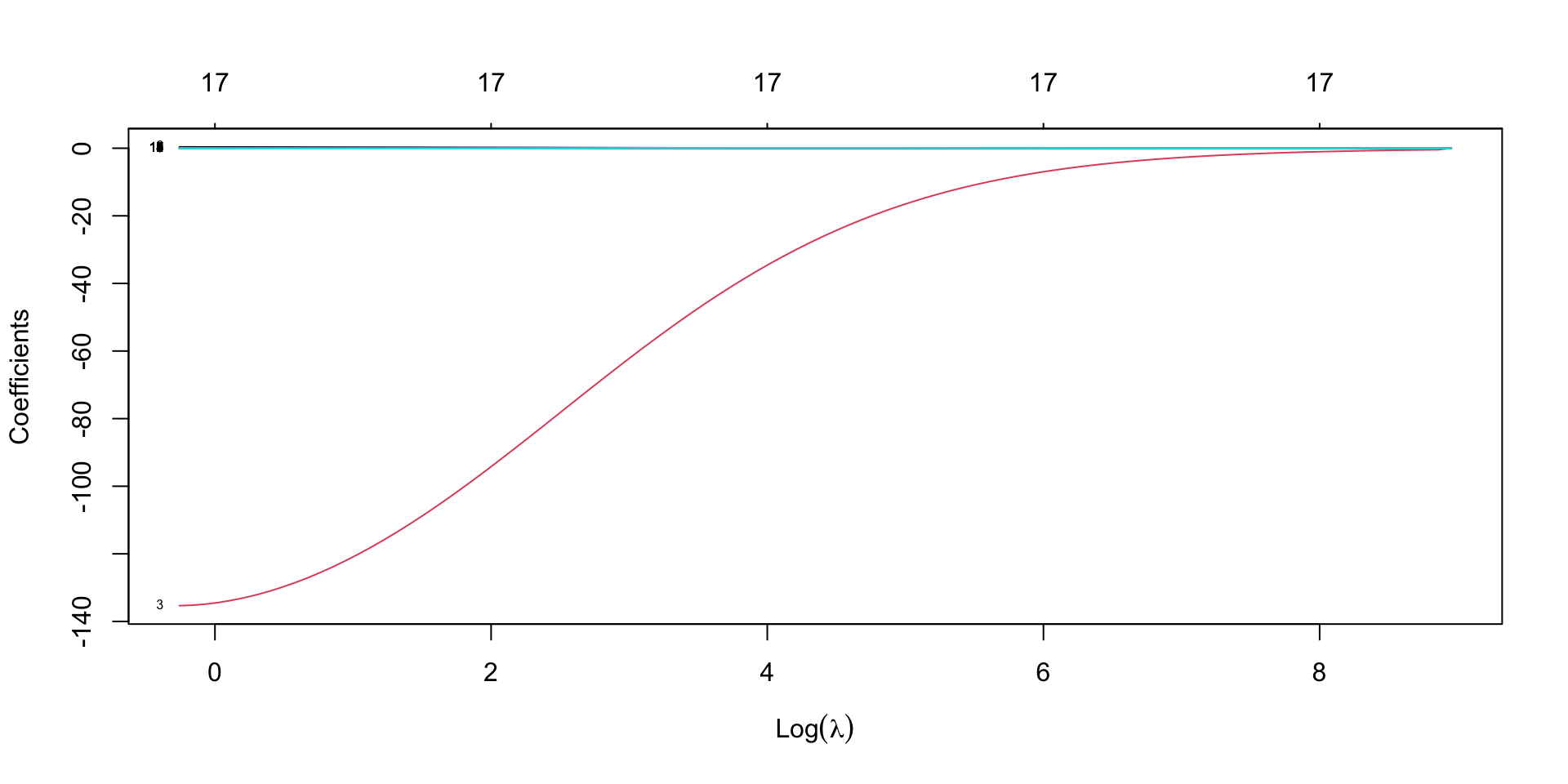
Ridge in R

library(glmnet)
library(UsingR)

# Prepare data
X <- model.matrix(body.fat ~ ., data = fat[, -1])
y <- fat$body.fat

# Fit ridge (alpha = 0)
ridge_mod <- glmnet(X, y, alpha = 0)

# Plot coefficient paths
plot(ridge_mod, xvar = "lambda", label = TRUE)

Choosing \(\lambda\): Cross-Validation

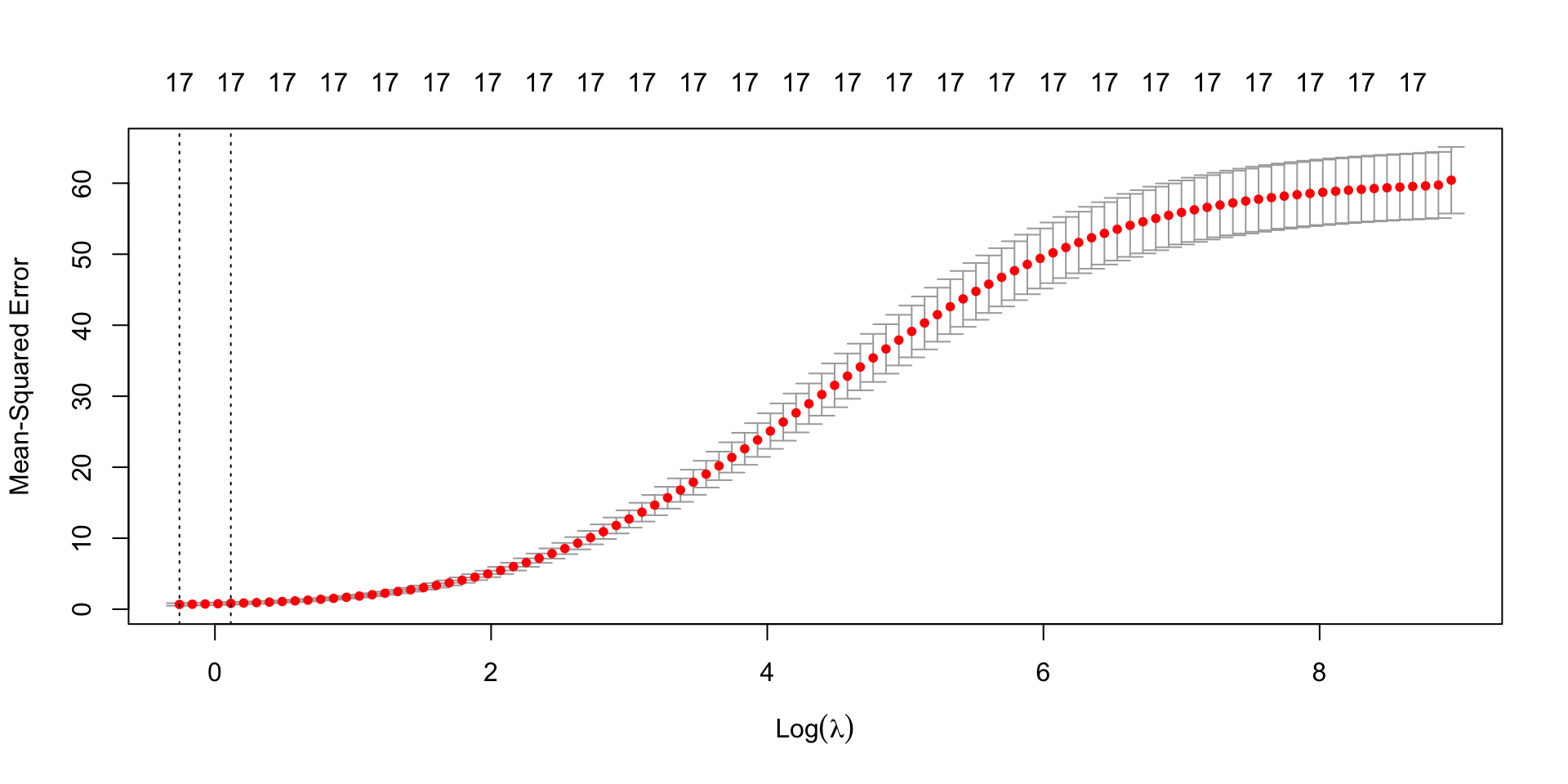
K-Fold Cross-Validation Steps:

Randomly divide data into \(K\) groups
For each \(\lambda\) value:
- Let group \(k\) be test data, rest be training
- Fit model on training data
- Predict test data and calculate error
Average error across all test sets
Select \(\lambda\) with minimum CV error

Cross-Validation in R

# Perform CV (default: 10-fold)
cv_ridge <- cv.glmnet(X, y, alpha = 0)

# Two common choices
lambda_min <- cv_ridge$lambda.min  # Minimum CV error
lambda_1se <- cv_ridge$lambda.1se  # 1 SE rule

# Plot CV results
plot(cv_ridge)

The Lasso

Least Absolute Shrinkage and Selection Operator

\[\sum_{i=1}^{n}(Y_i - \widehat{Y}_i)^2 + \lambda\sum_{k=1}^{p}|\beta_k|\]

Key difference: Uses absolute value penalty (\(L_1\) vs \(L_2\))

Why Use Lasso?

Sets coefficients exactly to zero (variable selection)
Creates sparse models (easier interpretation)
No closed-form solution (requires numerical optimization)

Tip

When to use:

Ridge: All variables are relevant
Lasso: Some variables are unnecessary

Lasso in R

# Fit Lasso (alpha = 1)
lasso_mod <- glmnet(X, y, alpha = 1)

# Cross-validation
cv_lasso <- cv.glmnet(X, y, alpha = 1)

# Refit with optimal lambda
final_mod <- glmnet(X, y, 
                    alpha = 1,
                    lambda = cv_lasso$lambda.1se)

# View coefficients
coef(final_mod)

19 x 1 sparse Matrix of class "dgCMatrix"
                      s0
(Intercept)    1.9827703
(Intercept)    .        
body.fat.siri  0.8985764
density       -0.2394245
age            .        
weight         .        
height         .        
BMI            .        
ffweight       .        
neck           .        
chest          .        
abdomen        .        
hip            .        
thigh          .        
knee           .        
ankle          .        
bicep          .        
forearm        .        
wrist          .

Ridge vs Lasso

Aspect	Ridge	Lasso
Penalty	\(L_2\) (squared)	\(L_1\) (absolute)
Variable selection	No	Yes
Coefficients	Shrink toward 0	Set to exactly 0
Solution	Closed form	Numerical
Best when	All variables relevant	Sparse truth

Example: Swiss Fertility Data

# Load data
data(swiss)

# Prepare matrices
X <- model.matrix(Fertility ~ ., swiss)[, -1]
y <- swiss$Fertility

# Fit OLS for comparison
lm(Fertility ~ ., data = swiss)


Call:
lm(formula = Fertility ~ ., data = swiss)

Coefficients:
     (Intercept)       Agriculture       Examination         Education  
         66.9152           -0.1721           -0.2580           -0.8709  
        Catholic  Infant.Mortality  
          0.1041            1.0770

Swiss Data: Ridge Results

# Ridge with CV
cv_ridge <- cv.glmnet(X, y, alpha = 0)

# Optimal lambda
ridge_final <- glmnet(X, y, 
                     alpha = 0,
                     lambda = cv_ridge$lambda.min)

coef(ridge_final)

6 x 1 sparse Matrix of class "dgCMatrix"
                          s0
(Intercept)      64.44211086
Agriculture      -0.12736848
Examination      -0.31867808
Education        -0.73073509
Catholic          0.08667922
Infant.Mortality  1.09634393

All 5 variables retained with shrunken coefficients

Swiss Data: Lasso Results

# Lasso with CV
cv_lasso <- cv.glmnet(X, y, alpha = 1)

# Optimal lambda (1 SE rule)
lasso_final <- glmnet(X, y,
                      alpha = 1, 
                      lambda = cv_lasso$lambda.1se)

coef(lasso_final)

6 x 1 sparse Matrix of class "dgCMatrix"
                          s0
(Intercept)      58.02076026
Agriculture       .         
Examination      -0.15340060
Education        -0.56041324
Catholic          0.05690564
Infant.Mortality  0.92578802

Agriculture set to 0; 4 variables selected

Example: Hitters Salary Data

library(ISLR2)

# Remove missing values
Hitters <- na.omit(Hitters)

# Check multicollinearity
cor(Hitters[, -c(14:15, 20)])  # High correlations!

            AtBat       Hits        HmRun        Runs        RBI     Walks
AtBat   1.0000000 0.96396913  0.555102154  0.89982910 0.79601539 0.6244481
Hits    0.9639691 1.00000000  0.530627358  0.91063014 0.78847819 0.5873105
HmRun   0.5551022 0.53062736  1.000000000  0.63107588 0.84910743 0.4404537
Runs    0.8998291 0.91063014  0.631075883  1.00000000 0.77869235 0.6970151
RBI     0.7960154 0.78847819  0.849107434  0.77869235 1.00000000 0.5695048
Walks   0.6244481 0.58731051  0.440453717  0.69701510 0.56950476 1.0000000
Years   0.0127255 0.01859809  0.113488420 -0.01197495 0.12966795 0.1347927
CAtBat  0.2071663 0.20667761  0.217463613  0.17181080 0.27812591 0.2694500
CHits   0.2253415 0.23560577  0.217495691  0.19132697 0.29213714 0.2707951
CHmRun  0.2124215 0.18936425  0.492525845  0.22970104 0.44218969 0.3495822
CRuns   0.2372778 0.23889610  0.258346846  0.23783121 0.30722616 0.3329766
CRBI    0.2213932 0.21938423  0.349858379  0.20233548 0.38777657 0.3126968
CWalks  0.1329257 0.12297073  0.227183183  0.16370021 0.23361884 0.4291399
PutOuts 0.3096075 0.29968754  0.250931497  0.27115986 0.31206456 0.2808555
Assists 0.3421174 0.30397495 -0.161601753  0.17925786 0.06290174 0.1025226
Errors  0.3255770 0.27987618 -0.009743082  0.19260879 0.15015469 0.0819372
Salary  0.3947709 0.43867474  0.343028078  0.41985856 0.44945709 0.4438673
              Years       CAtBat       CHits      CHmRun       CRuns
AtBat    0.01272550  0.207166254  0.22534146  0.21242155  0.23727777
Hits     0.01859809  0.206677608  0.23560577  0.18936425  0.23889610
HmRun    0.11348842  0.217463613  0.21749569  0.49252584  0.25834685
Runs    -0.01197495  0.171810798  0.19132697  0.22970104  0.23783121
RBI      0.12966795  0.278125914  0.29213714  0.44218969  0.30722616
Walks    0.13479270  0.269449974  0.27079505  0.34958216  0.33297657
Years    1.00000000  0.915680692  0.89784449  0.72237071  0.87664855
CAtBat   0.91568069  1.000000000  0.99505681  0.80167609  0.98274694
CHits    0.89784449  0.995056810  1.00000000  0.78665204  0.98454184
CHmRun   0.72237071  0.801676089  0.78665204  1.00000000  0.82562483
CRuns    0.87664855  0.982746941  0.98454184  0.82562483  1.00000000
CRBI     0.86380936  0.950730141  0.94679739  0.92790264  0.94567701
CWalks   0.83752373  0.906711655  0.89071842  0.81087827  0.92776846
PutOuts -0.02001921  0.053392514  0.06734799  0.09382223  0.05908718
Assists -0.08511772 -0.007897271 -0.01314420 -0.18888646 -0.03889509
Errors  -0.15651196 -0.070477521 -0.06803583 -0.16536941 -0.09408054
Salary   0.40065699  0.526135310  0.54890956  0.52493056  0.56267771
               CRBI      CWalks     PutOuts      Assists       Errors
AtBat    0.22139318  0.13292568  0.30960746  0.342117377  0.325576978
Hits     0.21938423  0.12297073  0.29968754  0.303974950  0.279876183
HmRun    0.34985838  0.22718318  0.25093150 -0.161601753 -0.009743082
Runs     0.20233548  0.16370021  0.27115986  0.179257859  0.192608787
RBI      0.38777657  0.23361884  0.31206456  0.062901737  0.150154692
Walks    0.31269680  0.42913990  0.28085548  0.102522559  0.081937197
Years    0.86380936  0.83752373 -0.02001921 -0.085117725 -0.156511957
CAtBat   0.95073014  0.90671165  0.05339251 -0.007897271 -0.070477521
CHits    0.94679739  0.89071842  0.06734799 -0.013144204 -0.068035829
CHmRun   0.92790264  0.81087827  0.09382223 -0.188886464 -0.165369407
CRuns    0.94567701  0.92776846  0.05908718 -0.038895093 -0.094080542
CRBI     1.00000000  0.88913701  0.09537515 -0.096558877 -0.115316131
CWalks   0.88913701  1.00000000  0.05816016 -0.066243445 -0.129935875
PutOuts  0.09537515  0.05816016  1.00000000 -0.043390143  0.075305857
Assists -0.09655888 -0.06624345 -0.04339014  1.000000000  0.703504693
Errors  -0.11531613 -0.12993587  0.07530586  0.703504693  1.000000000
Salary   0.56696569  0.48982204  0.30048036  0.025436136 -0.005400702
              Salary
AtBat    0.394770945
Hits     0.438674738
HmRun    0.343028078
Runs     0.419858559
RBI      0.449457088
Walks    0.443867260
Years    0.400656994
CAtBat   0.526135310
CHits    0.548909559
CHmRun   0.524930560
CRuns    0.562677711
CRBI     0.566965686
CWalks   0.489822036
PutOuts  0.300480356
Assists  0.025436136
Errors  -0.005400702
Salary   1.000000000

19 predictors with substantial multicollinearity

Hitters: Comparing Methods

OLS

All 19 variables
Many non-significant
High variance

Ridge

All 19 variables
Coefficients shrunken
Reduced variance

Lasso

8 variables selected
Sparse model
Better interpretation

Test Set Performance

# Split data
set.seed(1)
test_ind <- sample(1:nrow(Hitters), 20)
train <- Hitters[-test_ind, ]
test <- Hitters[test_ind, ]

# Compare test MSE (you first need to create all the _mod objects)
test_mse_ols <- mean((test$Salary - predict(ols_mod, test))^2)
test_mse_ridge <- mean((test$Salary - predict(ridge_mod, test))^2)
test_mse_lasso <- mean((test$Salary - predict(lasso_mod, test))^2)

Key Takeaways

Regularization addresses multicollinearity and overfitting
Ridge: Shrinks coefficients, keeps all variables
Lasso: Performs variable selection (sparse models)
Always use cross-validation to choose \(\lambda\)
Scale your variables before regularization!

Extensions

Elastic Net

Combines Ridge + Lasso: \(\alpha \in [0,1]\)
glmnet(X, y, alpha = 0.5)

Group Lasso

Select groups of variables together

Bayesian Interpretation

Ridge: Gaussian prior
Lasso: Laplace prior

Resources

R package: glmnet
Cross-validation: cv.glmnet()
ISLR Book Chapter 6
Always check ?glmnet for details

Practice

Try on your own data:

Check for multicollinearity
Fit both Ridge and Lasso with CV
Compare coefficient paths
Evaluate on test set
Interpret selected variables

🗓️ Week 09 Regularized Regression

Linear Regression Review

Ordinary Least Squares (OLS)

Common Issues with OLS

Ridge Regression

Bias-Variance Tradeoff

Ridge in Matrix Form

Ridge in R

Choosing \(\lambda\): Cross-Validation

Cross-Validation in R

The Lasso

Why Use Lasso?

Lasso in R

Ridge vs Lasso

Example: Swiss Fertility Data

Swiss Data: Ridge Results

Swiss Data: Lasso Results

Example: Hitters Salary Data

Hitters: Comparing Methods

Test Set Performance

Key Takeaways

Extensions

Resources

Practice

🗓️ Week 09
Regularized Regression