🗓️ Week 08
Clusters

STAT 204 – Introduction to Statistical Data Analysis

Prof. Marcela Alfaro Cordoba

Statistics - UCSC

18 Nov 2025

What is Cluster Analysis?

• Cluster analysis is a collection of techniques used to find clusters or subgroups in data
• The goal is to form groups that are homogeneous:
  • Observations within a subgroup are more similar to each other
  • Observations in different subgroups are more different from each other
• Relies on measures of similarity or dissimilarity
• It’s a type of unsupervised learning — we have data but no outcome labels

Cluster Analysis: Visual Intuition

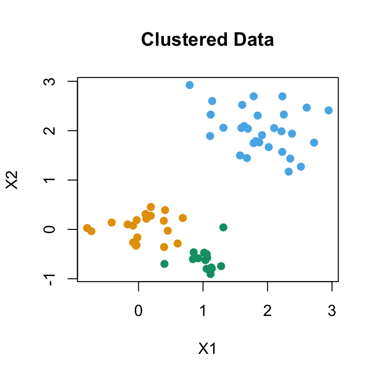
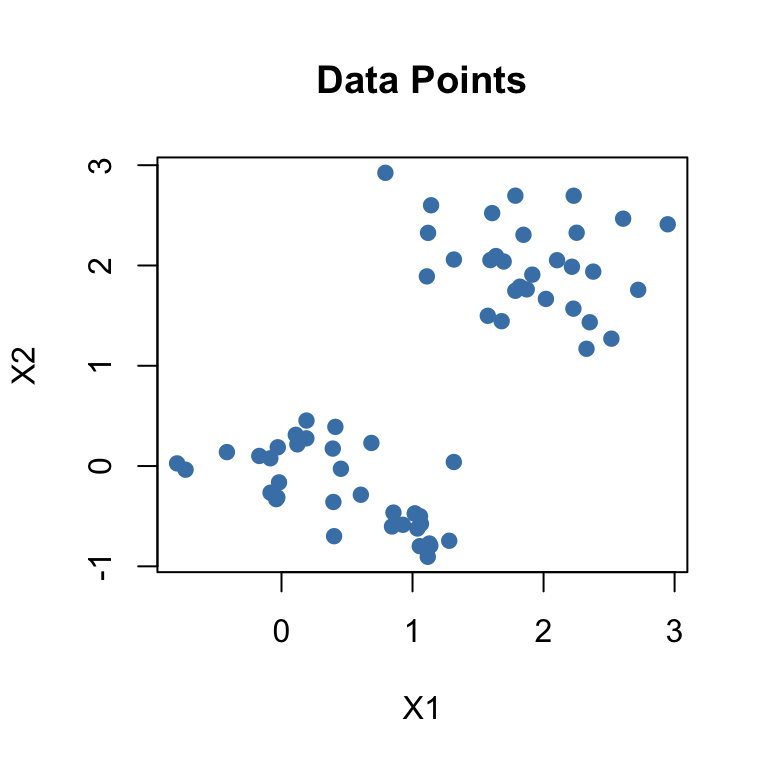
Raw data:

With clusters identified:

The algorithm discovers natural groupings in the data!

Supervised vs Unsupervised Learning

Supervised Learning (Classification)

• We have labeled data: observations have known group membership
• Goal: Build a model to predict labels for new observations
• Example: Classifying emails as spam or not spam

Unsupervised Learning (Clustering)

• We have unlabeled data: no predetermined groups
• Goal: Discover hidden patterns or structure in the data
• Example: Grouping customers by purchasing behavior

Note: Clustering can be used to create features for supervised learning!

Why Use Cluster Analysis?

Pattern detection: - Identify natural groupings in your data - Market segmentation (customer types) - Image segmentation - Document organization

Feature creation: - Create new categorical variables based on clusters - Use cluster membership as a predictor in other models

Data exploration: - Better understand the structure of your data - Generate hypotheses for further investigation

⚠️ Warning: Can also result in noise if patterns don’t really exist!

Common Clustering Algorithms

• K-means
• Hierarchical
• Others

• Partition observations into K pre-specified clusters
• Minimizes within-cluster variation
• Fast and widely used
• Requires choosing K in advance

• Builds a tree structure (dendrogram)
• Two approaches:
  • Agglomerative: Start with each point as its own cluster, merge
  • Divisive: Start with one cluster, split
• Don’t need to specify number of clusters upfront
• Can choose K by “cutting” the tree

• K-medoids
• DBSCAN
• Mixture models
• Spectral clustering

Distance/Dissimilarity Measures

Given two observations \(\mathbf{x}_i\) and \(\mathbf{x}_{i'}\), a dissimilarity measure \(d_{ii'}\) must satisfy:

1. \(d_{ii'} \geq 0\) for all observations \(\mathbf{x}_i\) and \(\mathbf{x}_{i'}\)
2. \(d_{ii'} = 0\) if and only if \(\mathbf{x}_i = \mathbf{x}_{i'}\)
3. \(d_{ii'} = d_{i'i}\) (symmetry)

We typically construct the proximity matrix \(\mathbf{D}\), an \(n \times n\) matrix where element \((i, i')\) is \(d_{ii'}\)

Common Distance Measures

Euclidean distance (most common): \(d_{ii'} = \sqrt{\sum_{j=1}^p (x_{ij} - x_{i'j})^2}\)

Minkowski metric (generalization): \[d_{ii'} = \left(\sum_{j=1}^p |x_{ij} - x_{i'j}|^\lambda\right)^{1/\lambda}\]

where \(\lambda = 2\) gives Euclidean distance, \(\lambda = 1\) gives Manhattan distance

Important!

Make sure to scale your variables if they’re on different units/scales!

K-means Clustering

K-means as an Optimization Problem

K-means tries to minimize the within-cluster sum of squares:

\[\text{minimize} \sum_{k=1}^K \sum_{C(i)=k} \sum_{C(i')=k} d(\mathbf{x}_i, \mathbf{x}_{i'})\]

In words: minimize the sum over all clusters of the total distances between points within each cluster

With Euclidean distance, this is equivalent to minimizing: \[\sum_{k=1}^K \sum_{C(i)=k} \|\mathbf{x}_i - \bar{\mathbf{x}}_k\|^2\]

where \(\bar{\mathbf{x}}_k\) is the centroid (mean) of cluster \(k\)

The K-means Algorithm

Algorithm

1. Initialize: Randomly assign each observation to one of K clusters

2. Iterate until convergence:

   1. For each cluster \(k\), compute the cluster centroid \(\bar{\mathbf{x}}_k\) (the vector of column means)

   2. Assign each observation to the cluster with the closest centroid

The algorithm converges when cluster assignments stop changing

Note

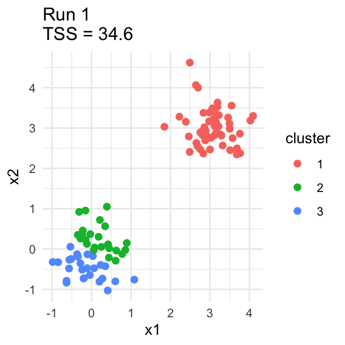
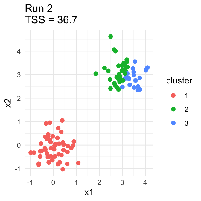
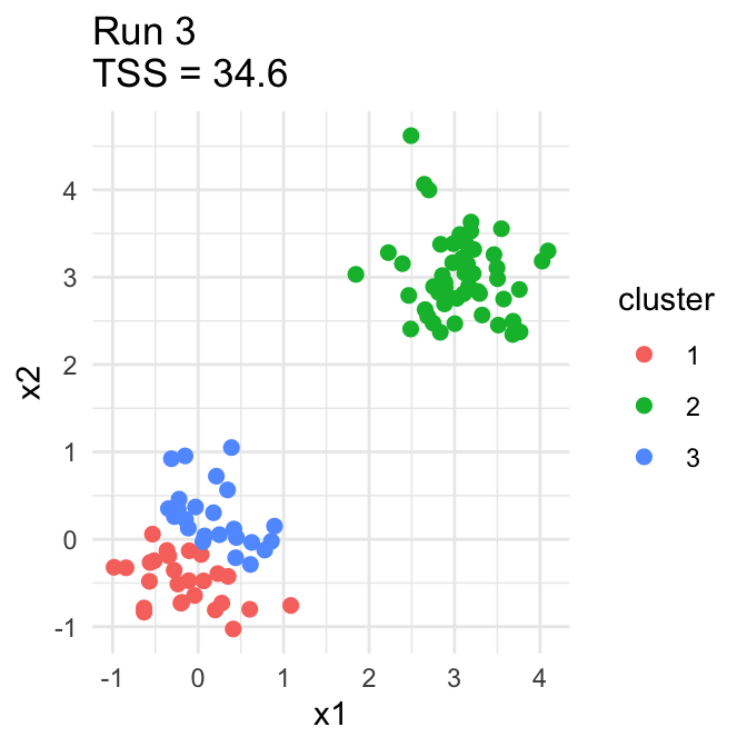
Convergence: The algorithm is guaranteed to converge, but not necessarily to the global optimum — only to a local minimum!

K-means Example: Iteration 1

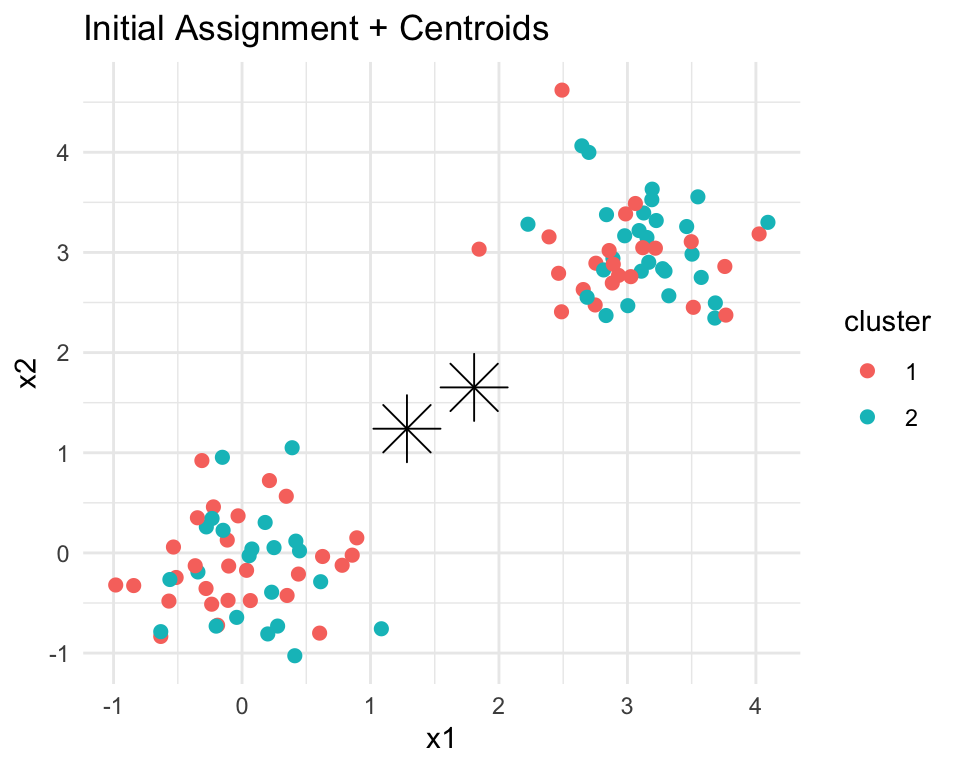
Initial random assignment:

After reassignment:

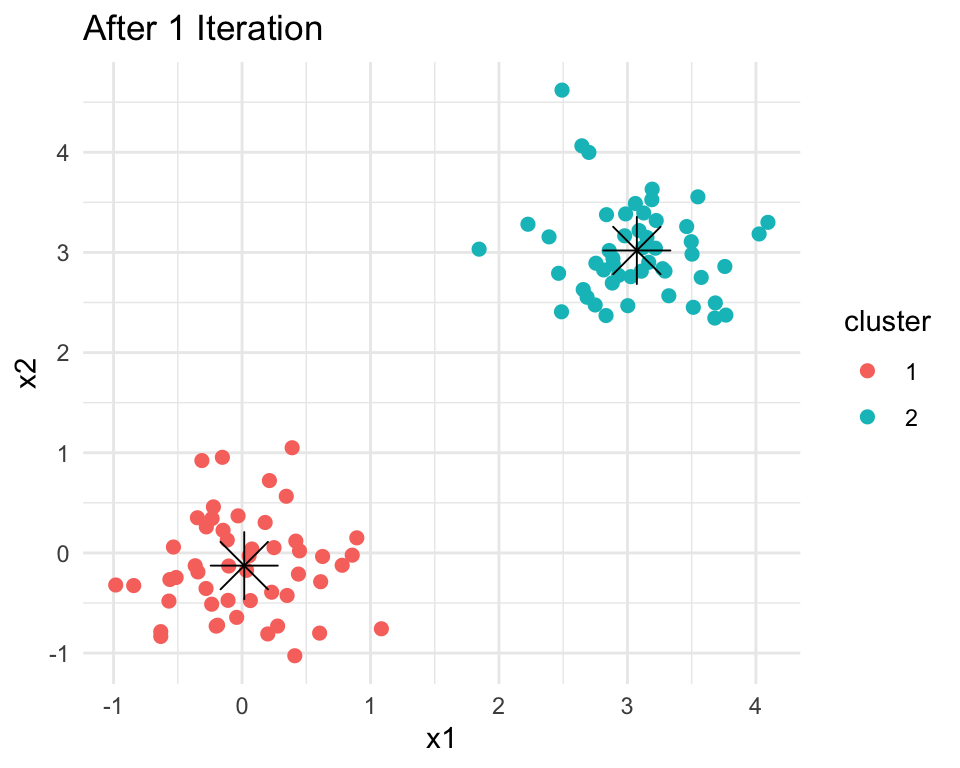
⭐ Stars show cluster centroids

K-means: Local Minima Problem

Solution: Run the algorithm multiple times with different random starts and pick the best solution!

K-means in R: Swiss Data Example

# Swiss fertility data
head(swiss, 3)

             Fertility Agriculture Examination Education Catholic
Courtelary        80.2        17.0          15        12     9.96
Delemont          83.1        45.1           6         9    84.84
Franches-Mnt      92.5        39.7           5         5    93.40
             Infant.Mortality
Courtelary               22.2
Delemont                 22.2
Franches-Mnt             20.2

# K-means with K=3, using 10 random starts
set.seed(10)
kmeans_swiss <- kmeans(swiss, centers=3, nstart=10)

# Cluster assignments
head(kmeans_swiss$cluster)

  Courtelary     Delemont Franches-Mnt      Moutier   Neuveville   Porrentruy 
           1            3            3            2            2            3 

K-means Results: Cluster Centers

# Cluster centers (means for each variable in each cluster)
kmeans_swiss$centers

  Fertility Agriculture Examination Education Catholic Infant.Mortality
1  58.30909    19.50909    25.72727    23.000 22.21455         19.22727
2  68.32500    55.90500    17.05000     7.850  7.55000         19.67000
3  80.55000    65.51875     9.43750     6.625 96.15000         20.77500

Interpretation

• Cluster 1:
• Cluster 2:
  
• Cluster 3:

Add your interpretations on Ed Discussion

Visualizing Clusters with PCA

library(ggplot2)
# Project onto first 2 principal components for visualization
pc_swiss <- prcomp(swiss)
plotDF <- data.frame(
  PC1 = pc_swiss$x[,1],
  PC2 = pc_swiss$x[,2],
  Cluster = factor(kmeans_swiss$cluster)
)

ggplot(plotDF, aes(x=PC1, y=PC2, color=Cluster)) + 
  geom_point(size=3) + 
  theme_minimal() +
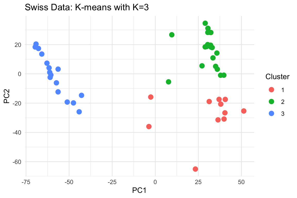
  labs(title="Swiss Data: K-means with K=3")

K-means: Penguins Example

The penguins dataset has known species labels — let’s see if K-means can recover them!

library(dplyr)
library(palmerpenguins)
# Prepare data: select variables and remove missing values
penguins_clean <- penguins %>%
  dplyr::select(bill_length_mm, bill_depth_mm,
  flipper_length_mm, body_mass_g, sex, species) %>%
  na.omit()
# Standardize the numeric variables
penguins_scaled <- penguins_clean %>%
  mutate(across(c(bill_length_mm, bill_depth_mm, 
  flipper_length_mm, body_mass_g), scale))
# Convert sex to numeric (0/1) for clustering
penguins_for_clustering <- penguins_scaled %>%
  mutate(sex_numeric = as.numeric(sex) - 1) %>%
  select(bill_length_mm, bill_depth_mm, flipper_length_mm, 
  body_mass_g, sex_numeric)
# Run K-means with K=3 (there are 3 penguin species)
set.seed(1)
km_penguins <- kmeans(penguins_for_clustering, centers=3, nstart=10)
# Compare clusters to true species
table(Cluster = km_penguins$cluster, Species = penguins_clean$species)

       Species
Cluster Adelie Chinstrap Gentoo
      1     25        61      0
      2      0         0    119
      3    121         7      0

Not perfect, but pretty good! Clusters 2 and 3 mostly separate Gentoo and Adelie.

Choosing K: The Elbow Method

How do we choose K? Try multiple values and look for an “elbow” in the plot:

# Try K from 2 to 10
set.seed(1)
tss_values <- sapply(2:10, function(k) {
  km <- kmeans(swiss, centers=k, nstart=10)
  km$tot.withinss
})

plot(2:10, tss_values, type='b', 
     xlab="Number of Clusters (K)", 
     ylab="Total Within-Cluster SS",
     main="Elbow Method for Choosing K", pch=19)

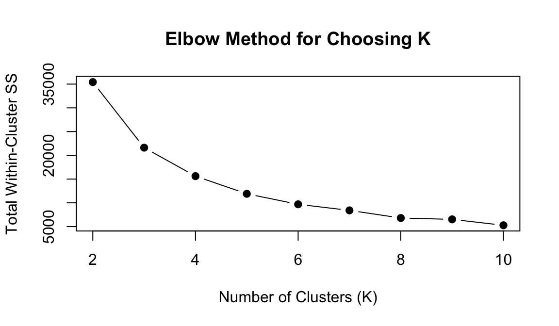
Look for where the decrease starts to level off — here maybe K=3 or K=4?

K-means Limitations

Limitation 1: Must specify K

You need to decide on the number of clusters beforehand (though the elbow method can help)

Limitation 2: Assumes spherical clusters

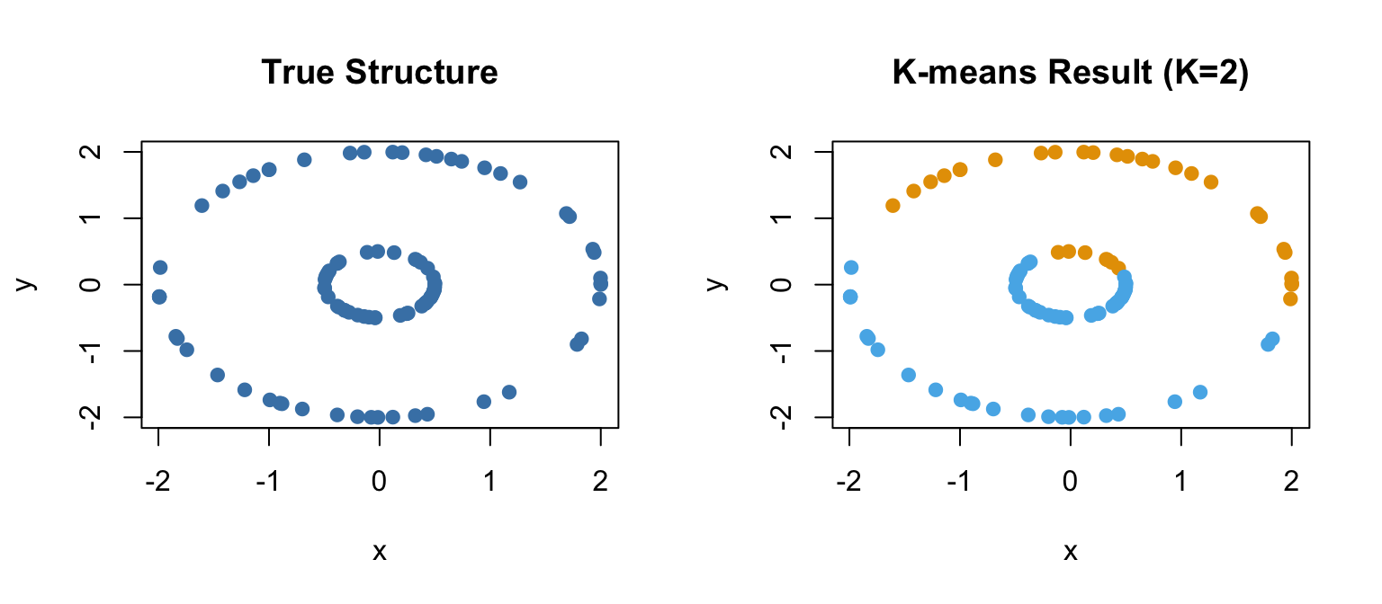
K-means works best when clusters are roughly circular/spherical — it can fail on complex shapes

Limitation 3: Sensitive to outliers

Centroids can be pulled by extreme values

Limitation 4: Scale matters

Variables with larger scales dominate — always standardize!

When K-means Fails: Non-spherical Clusters

K-means struggles with non-convex shapes! Other methods (e.g., DBSCAN) work better here.

Hierarchical Clustering

What is Hierarchical Clustering?

• Doesn’t require specifying K upfront!
• Builds a tree structure (dendrogram) showing how observations are grouped
• Two main approaches:
  • Agglomerative (bottom-up): Start with each point in its own cluster, then merge
  • Divisive (top-down): Start with all points in one cluster, then split
• We’ll focus on agglomerative clustering (most common)

Understanding Dendrograms

Key features:

• Each leaf = one observation
• Height of merge = dissimilarity between clusters
• Taller merges = more different clusters
• Cut the tree at different heights to get different numbers of clusters

Agglomerative Clustering Algorithm

Algorithm

1. Start with \(n\) clusters (each observation is its own cluster)

2. Repeat until only one cluster remains:

   1. Compute all pairwise inter-cluster dissimilarities

   2. Identify the two clusters that are most similar

   3. Merge these two clusters

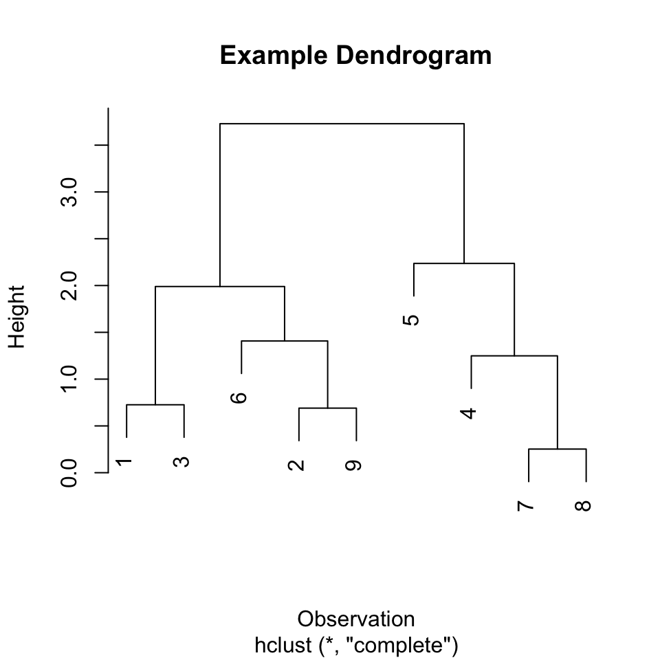
   4. Record the height (dissimilarity) at which the merge occurs

The result is a dendrogram!

Linkage Methods

How do we measure dissimilarity between clusters? Different linkage methods:

• Complete
• Single
• Average
• Centroid

Maximum dissimilarity between any two points in the clusters

\[d_{\text{complete}}(A, B) = \max_{i \in A, i' \in B} d_{ii'}\]

Most popular; tends to produce compact clusters

Minimum dissimilarity between any two points in the clusters

\[d_{\text{single}}(A, B) = \min_{i \in A, i' \in B} d_{ii'}\]

Can produce “chaining” (long, stretched clusters)

Mean of all pairwise dissimilarities

\[d_{\text{average}}(A, B) = \frac{1}{|A||B|}\sum_{i \in A}\sum_{i' \in B} d_{ii'}\]

Compromise between single and complete

Dissimilarity between cluster centroids

Can sometimes lead to inversions (not monotonic)

Linkage Comparison: Same Data, Different Results

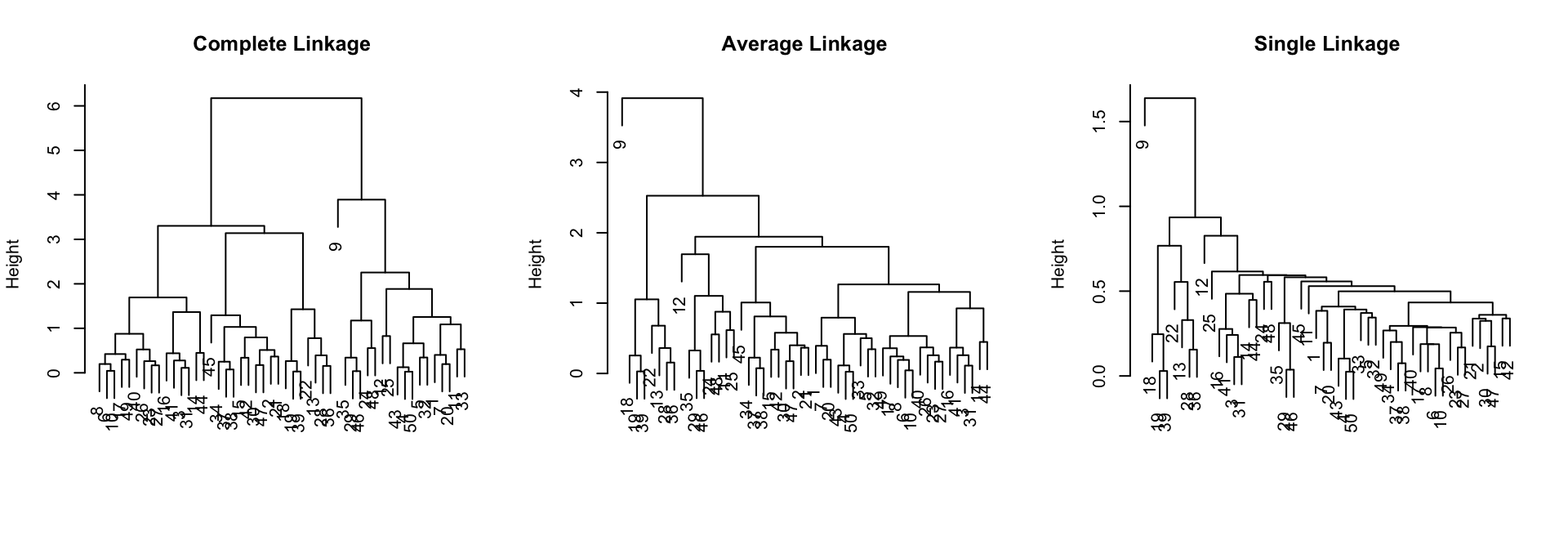
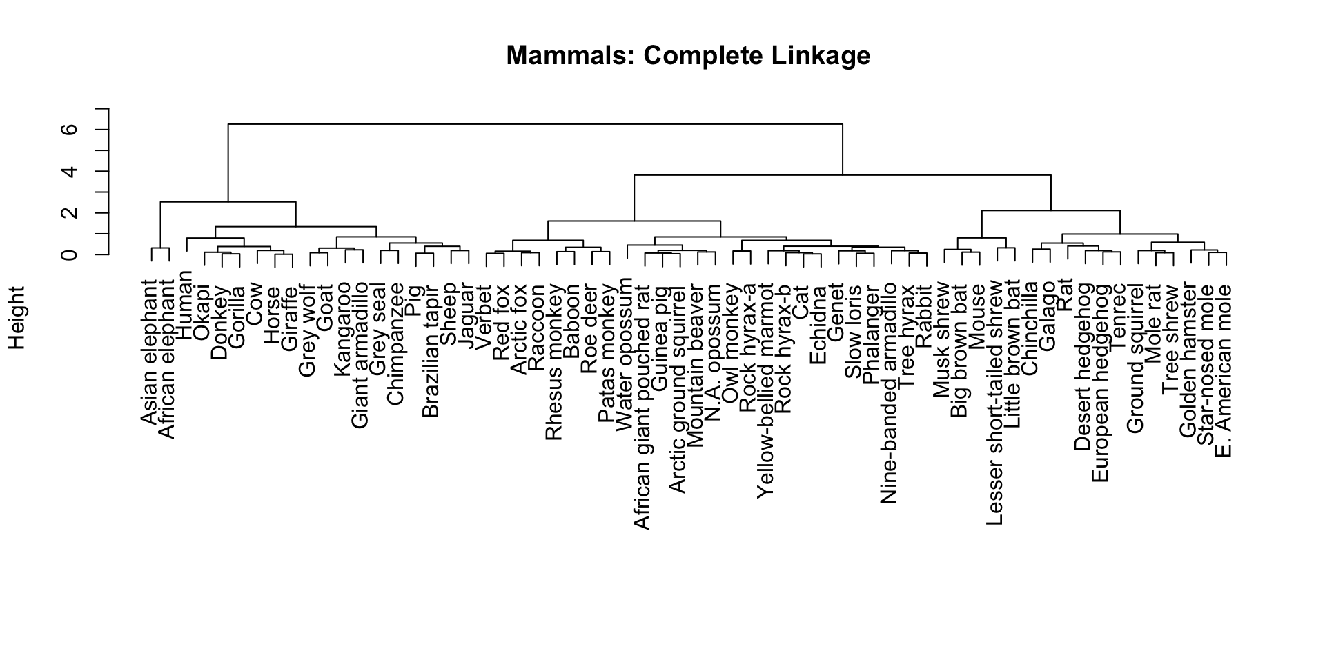
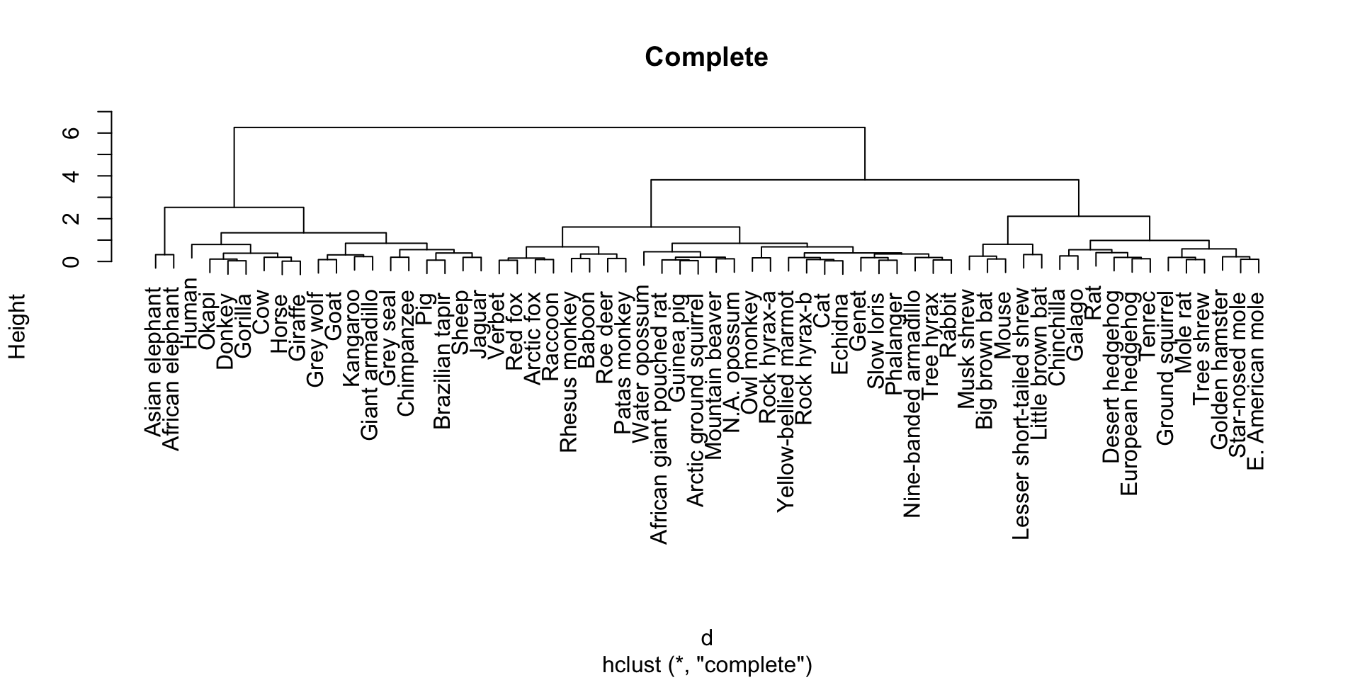
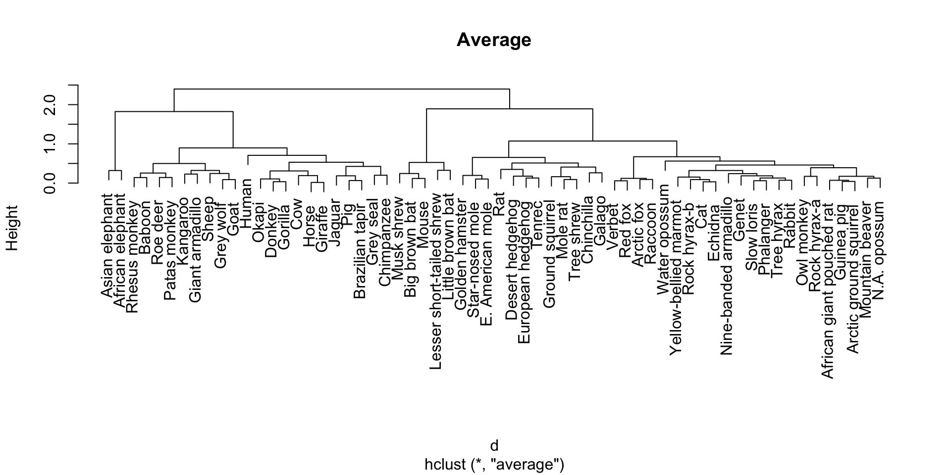
Different linkage methods can give very different tree structures!

Hierarchical Clustering in R

# Load mammals data
library(MASS)
head(mammals, 3)

                 body brain
Arctic fox      3.385  44.5
Owl monkey      0.480  15.5
Mountain beaver 1.350   8.1

# Compute distance matrix on log scale
d <- dist(scale(log(mammals)))

# Hierarchical clustering with complete linkage
hc_complete <- hclust(d, method="complete")

Dendrogram: Mammals Example

plot(hc_complete, main="Mammals: Complete Linkage", xlab="", sub="")

Extracting Clusters from Dendrogram

Use cutree() to cut the dendrogram at different heights or to get K clusters:

# Get 3 clusters
clusters_3 <- cutree(hc_complete, k=3)
table(clusters_3)

clusters_3
 1  2  3 
26 19 17 

# Get 5 clusters
clusters_5 <- cutree(hc_complete, k=5)
table(clusters_5)

clusters_5
 1  2  3  4  5 
26 17 12  5  2 

Comparing Different Linkage Methods

Complete linkage:

plot(hc_complete, main="Complete")

Comparing Different Linkage Methods

Average linkage:

hc_avg <- hclust(d, method="average")
plot(hc_avg, main="Average")

Tree structures can look quite different!

Protein Consumption Example

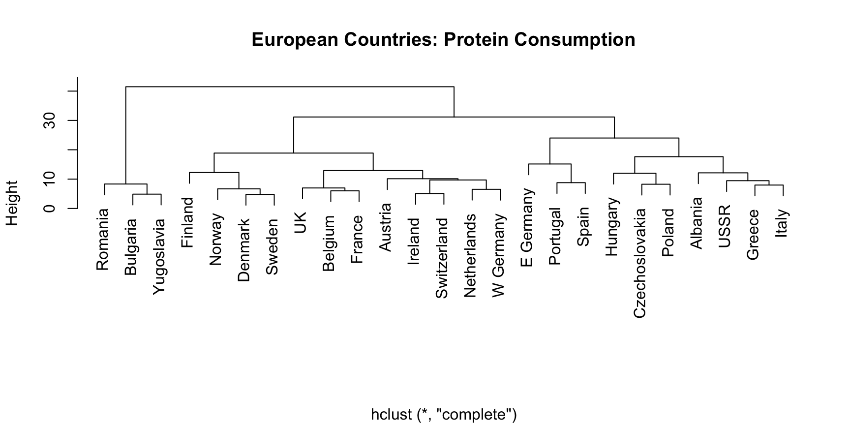
European countries grouped by protein consumption patterns:

food <- read.csv('http://www.biz.uiowa.edu/faculty/jledolter/DataMining/protein.csv')
rownames(food) <- food[,1]
d_food <- dist(food[,-1])
hc_food <- hclust(d_food, method="complete")
plot(hc_food, main="European Countries: Protein Consumption", xlab="")

Hierarchical vs K-means

Feature	K-means	Hierarchical
Choose K?	✅ Yes, upfront	❌ No, choose later from dendrogram
Computational	✅ Fast, scalable	⚠️ Slower for large data
Deterministic?	❌ No, random starts	✅ Yes (given distance)
Visual	Scatter plot	Dendrogram tree
Cluster shapes	Spherical/convex	More flexible

Recommendation

Try both methods and compare results! They often give complementary insights.

Practical Considerations

Scaling Variables is Critical!

Problem: Variables on different scales dominate the clustering

# Before scaling
head(penguins_clean, 2)

# A tibble: 2 × 6
  bill_length_mm bill_depth_mm flipper_length_mm body_mass_g sex    species
           <dbl>         <dbl>             <int>       <int> <fct>  <fct>  
1           39.1          18.7               181        3750 male   Adelie 
2           39.5          17.4               186        3800 female Adelie 

# After scaling
penguins_scaled <- penguins_clean %>%
  mutate(across(c(bill_length_mm, bill_depth_mm, 
  flipper_length_mm, body_mass_g), scale))
head(penguins_scaled, 2)

# A tibble: 2 × 6
  bill_length_mm[,1] bill_depth_mm[,1] flipper_length_mm[,1] body_mass_g[,1]
               <dbl>             <dbl>                 <dbl>           <dbl>
1             -0.895             0.780                 -1.42          -0.568
2             -0.822             0.119                 -1.07          -0.506
# ℹ 2 more variables: sex <fct>, species <fct>

Always standardize unless you have a good reason not to!

Handling Missing Values

Clustering algorithms typically can’t handle missing data directly.

Options:

1. Remove observations with missing values (if not too many)

data_complete <- na.omit(data)

2. Impute missing values before clustering

# Simple imputation with median
data$var[is.na(data$var)] <- median(data$var, na.rm=TRUE)

3. Use algorithms designed for missing data (more advanced)

Validating Clusters

Important Question

How do we know if our clusters are “real” or just artifacts?

Approaches:

1. Silhouette analysis: Measures how similar each point is to its own cluster vs other clusters

2. Gap statistic: Compares within-cluster variation to a null reference distribution

3. Domain knowledge: Do the clusters make sense? Can you interpret them?

4. Stability: Do you get similar results with different random samples?

Warning

Clustering can find patterns in random data! Always be skeptical and validate.

Curse of Dimensionality

Problem: In high dimensions, all distances become similar!

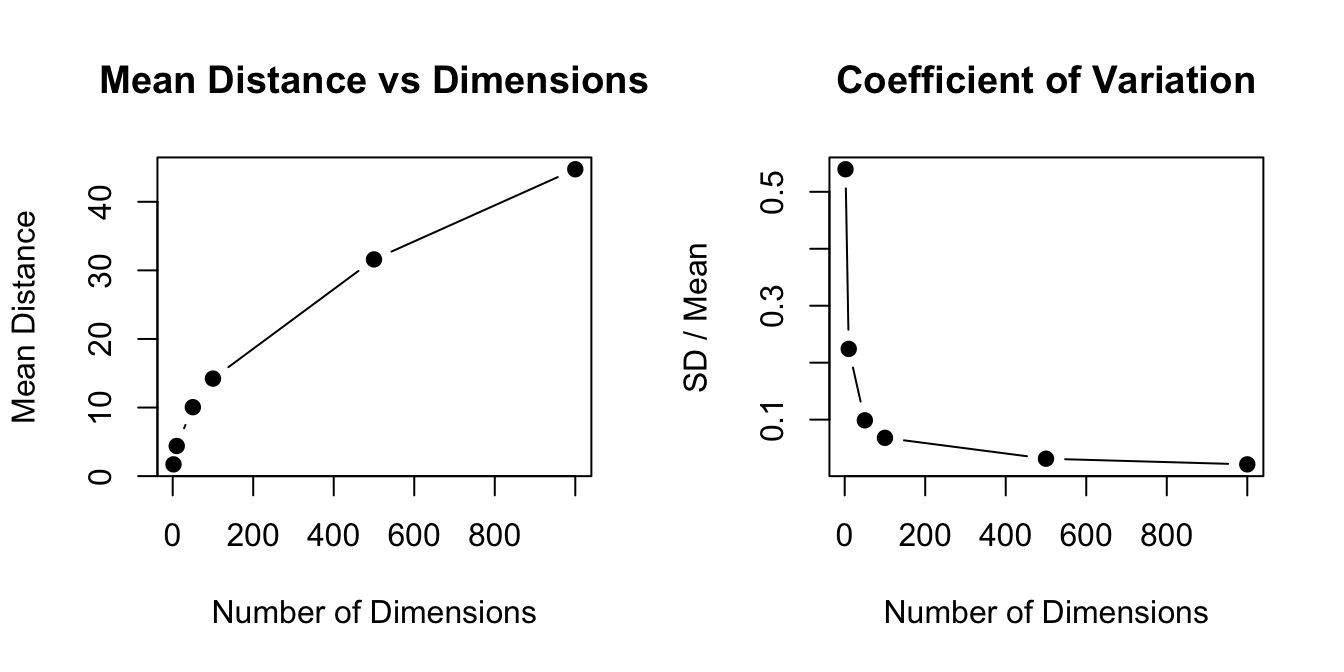
Solutions: Dimension reduction (PCA) before clustering, or use algorithms designed for high dimensions

Example: MNIST Digits

Can K-means separate handwritten 0s and 1s?

# Each image is 28x28 = 784 pixels
digits <- read.csv('data/digits.csv')
labels <- read.csv('data/digitsLabel.csv')
X <- as.matrix(digits[,-1])

set.seed(1)
km <- kmeans(X, centers=2, nstart=10)
table(Cluster = km$cluster, True_Label = labels$x)

       True_Label
Cluster    0    1
      1   10 1135
      2  970    0

Almost perfect separation! (Without using any labels during training)

Clustering on Principal Components

Often works well to:

1. First: Run PCA to reduce dimensionality
2. Then: Cluster on the first few PCs

# Run PCA first
X_pca <- prcomp(X, rank.=10)$x  # Keep 10 PCs

# Then cluster
km_pca <- kmeans(X_pca, centers=2, nstart=10)

Benefits: Faster, more stable, avoids curse of dimensionality

Other Clustering Methods

Beyond K-means and hierarchical:

• K-medoids (PAM): More robust to outliers than K-means
• DBSCAN: Density-based, good for non-convex shapes
• Gaussian Mixture Models: Probabilistic, soft clustering
• Spectral clustering: Uses graph theory, good for complex structures
• Fuzzy clustering: Observations can belong to multiple clusters
• Time series clustering: Special methods for temporal data

Each method has strengths and weaknesses — choose based on your data and goals!

Summary: Key Takeaways

What We Learned

✅ Clustering is unsupervised learning — finding groups without labels

✅ K-means: Fast, but requires choosing K and assumes spherical clusters

✅ Hierarchical: Flexible, creates dendrogram, linkage method matters

✅ Distance matters: Scale your variables, choose appropriate metric

✅ Validation is crucial: Don’t trust clusters blindly!

✅ Real-world tips: - Try multiple methods and compare - Use domain knowledge to interpret results - Consider dimension reduction first for high-dimensional data

References and Resources

Books:

• Hastie et al., The Elements of Statistical Learning (Chapter 14.3)

R Packages:

• stats: kmeans(), hclust(), cutree()
• cluster: More advanced methods. See R Package
• factoextra: Visualization tools. See R Package

Online:

• UC Business Analytics: Clustering
• StatQuest: Hierarchical Clustering

Practice Problems

Try These:

1. Load the USArrests dataset and perform K-means clustering with K=3. Interpret the clusters.

2. Use hierarchical clustering on the same data with different linkage methods. How do results differ?

3. Apply the elbow method to determine the optimal number of clusters.

4. Create a dendrogram and color different branches based on cluster membership.

5. Compare clustering results on raw vs. scaled data. What changes?

Questions?

Thank you!