🗓️ Week 07
Principal Component Analysis (PCA)

STAT 204 – Introduction to Statistical Data Analysis

Prof. Marcela Alfaro Cordoba

Statistics - UCSC

13 Nov 2025

Class Overview

Today’s Focus:

What is Principal Component Analysis and when to use it
Understanding covariance and correlation matrices
The mathematical foundation: eigenvalues and eigenvectors
Performing PCA in R
Interpreting loadings and scores
Determining how many components to retain
Practical applications of PCA

Learning Goals: Master dimensionality reduction and understand variance structure in multivariate data

Motivation: The Curse of Dimensionality

Consider a dataset with many variables:

Student performance: 100 test questions
Gene expression: 20,000 genes measured
Image data: 784 pixels (28×28 image)
Survey responses: 50 questions

Problems with high-dimensional data:

Hard to visualize
Computationally expensive
Many variables are correlated (redundant information)
Overfitting in predictive models

Question: Can we reduce dimensions while preserving information?

Why Do We Need PCA?

Real-world example: Suppose you measure students on:

Algebra score
Geometry score
Calculus score
Statistics score
Probability score

Key insight: These scores are likely highly correlated!

Students good at algebra tend to be good at calculus
High correlation means redundant information
Maybe we can capture most variation with fewer variables?

Why Do We Need PCA?

Real-world example: Suppose you measure students on:

Algebra score
Geometry score
Calculus score
Statistics score
Probability score

PCA finds new variables (principal components) that:

Are uncorrelated with each other
Capture maximum variance in the data
Are linear combinations of original variables

What Exactly Does PCA Do?

PCA creates new variables (components) as weighted combinations:

\[PC_1 = w_{11}X_1 + w_{12}X_2 + \cdots + w_{1p}X_p\]

\[PC_2 = w_{21}X_1 + w_{22}X_2 + \cdots + w_{2p}X_p\]

Key properties:

PC1 captures the most variance possible
PC2 captures the second most variance, uncorrelated with PC1
Each subsequent PC captures remaining variance
PCs are orthogonal (uncorrelated)

Result: Often the first few PCs capture most of the variance!

Our Running Example: Test Scores

Dataset: 88 students taking 5 exams

library(bootstrap)
data(scor)
head(scor, 10)

   mec vec alg ana sta
1   77  82  67  67  81
2   63  78  80  70  81
3   75  73  71  66  81
4   55  72  63  70  68
5   63  63  65  70  63
6   53  61  72  64  73
7   51  67  65  65  68
8   59  70  68  62  56
9   62  60  58  62  70
10  64  72  60  62  45

mec: Mechanics exam
vec: Vectors exam
alg: Algebra exam
ana: Analysis exam
sta: Statistics exam

Exploring Correlations

Before PCA, let’s examine correlations:

# Correlation matrix
cor(scor)

          mec       vec       alg       ana       sta
mec 1.0000000 0.5534052 0.5467511 0.4093920 0.3890993
vec 0.5534052 1.0000000 0.6096447 0.4850813 0.4364487
alg 0.5467511 0.6096447 1.0000000 0.7108059 0.6647357
ana 0.4093920 0.4850813 0.7108059 1.0000000 0.6071743
sta 0.3890993 0.4364487 0.6647357 0.6071743 1.0000000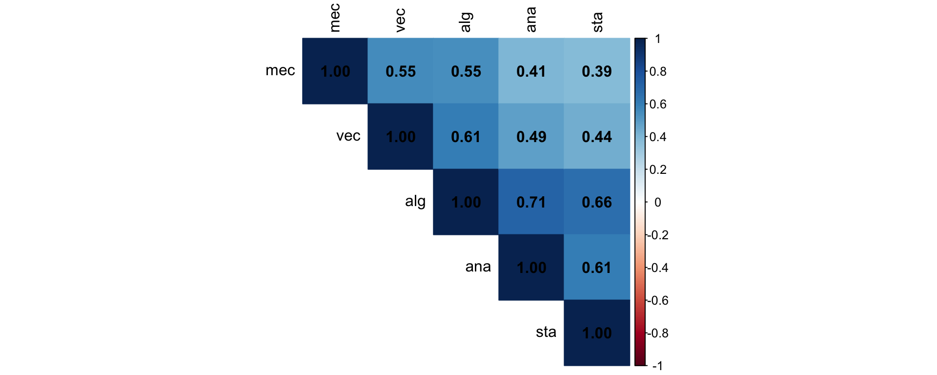

# Visualize
library(corrplot)
corrplot(cor(scor), method = "color", type = "upper", 
         addCoef.col = "black", tl.col = "black")

Observations: All exams positively correlated - students who do well on one tend to do well on others!

The Mathematics Behind PCA

PCA is based on eigendecomposition of the covariance matrix:

\[\Sigma = A\Lambda A'\]

where:

\(\Sigma\) is the \(p \times p\) covariance matrix
\(A\) is a matrix whose columns are eigenvectors (the PC loadings)
\(\Lambda\) is a diagonal matrix containing eigenvalues
\(A'A = I\) (eigenvectors are orthonormal)

Key insight:

The \(j\)-th eigenvector gives the weights for \(PC_j\)
The \(j\)-th eigenvalue equals the variance of \(PC_j\)
Eigenvalues are ordered: \(\lambda_1 \geq \lambda_2 \geq \cdots \geq \lambda_p \geq 0\)

Eigen Decomposition Reference

Covariance vs. Correlation Matrix

Two approaches for PCA:

1. Covariance matrix (\(\Sigma\)):

Uses original units of variables
Variables with larger variance dominate
Use when variables measured in same units
prcomp(data, scale = FALSE) uses covariance

2. Correlation matrix (standardized):

Standardizes all variables to mean 0, variance 1
Treats all variables equally
Use when variables have different units/scales
prcomp(data, scale = TRUE) uses correlation

Performing PCA in R

For test scores: We’ll use correlation since scores may have different scales!

# Perform PCA (using correlation matrix)
pca_result <- prcomp(scor, scale = TRUE)

# What's in the output?
names(pca_result)

[1] "sdev"     "rotation" "center"   "scale"    "x"

Components of output:

sdev: Standard deviations of each PC (sqrt of eigenvalues)
rotation: PC loadings (eigenvectors) - the weights
center: Original variable means
scale: Original variable standard deviations
x: PC scores - the transformed data

Understanding PC Loadings

Loadings show how original variables combine to create PCs:

pca_result$rotation

           PC1        PC2         PC3        PC4        PC5
mec -0.3996045 -0.6454583  0.62078249 -0.1457865 -0.1306722
vec -0.4314191 -0.4415053 -0.70500628  0.2981351 -0.1817479
alg -0.5032816  0.1290675 -0.03704901 -0.1085987  0.8466894
ana -0.4569938  0.3879057 -0.13618182 -0.6662561 -0.4221885
sta -0.4382444  0.4704545  0.31253342  0.6589164 -0.2340223

Interpretation of PC1 (first column):

All loadings negative and similar magnitude (~-0.4 to -0.5)
PC1 = -0.40(mec) - 0.43(vec) - 0.50(alg) - 0.46(ana) - 0.44(sta)
As PC1 increases, all exam scores decrease
PC1 represents overall poor performance (or negative overall ability)
Students with high PC1 scores did poorly across all exams

Interpreting PC2

# Look at PC2 specifically
pca_result$rotation[, 2]

       mec        vec        alg        ana        sta 
-0.6454583 -0.4415053  0.1290675  0.3879057  0.4704545

Interpretation of PC2:

Negative weights: mec (-0.65), vec (-0.44)
Positive weights: alg (+0.13), ana (+0.39), sta (+0.47)

As PC2 increases:

Performance on mec/vec decreases
Performance on alg/ana/sta increases

Meaning: PC2 contrasts mechanics/vectors performance against algebra/analysis/statistics performance - a math type dimension!

Variance Explained by Each PC

How much variance does each PC capture?

# Eigenvalues (variances)
eigenvalues <- pca_result$sdev^2
eigenvalues

[1] 3.1809801 0.7395718 0.4449651 0.3878924 0.2465905

# Proportion of variance
prop_var <- eigenvalues / sum(eigenvalues)
prop_var

[1] 0.63619603 0.14791437 0.08899303 0.07757848 0.04931810

# Cumulative proportion
cumsum(prop_var)

[1] 0.6361960 0.7841104 0.8731034 0.9506819 1.0000000

Key findings:

PC1 explains 63.6% of total variance
PC2 explains 14.8% additional variance
First 2 PCs together explain 78.4% of variance!

Visualizing Variance Explained: Scree Plot

Scree plot shows variance by component:

# Method 1: Using base R
screeplot(pca_result, type = "lines", main = "Scree Plot")

# Method 2: Manual plot
plot(1:5, eigenvalues, type = "b", 
     xlab = "Principal Component", 
     ylab = "Variance (Eigenvalue)",
     main = "Scree Plot", pch = 19, col = "blue")
abline(h = 1, lty = 2, col = "red")  # Kaiser criterion line

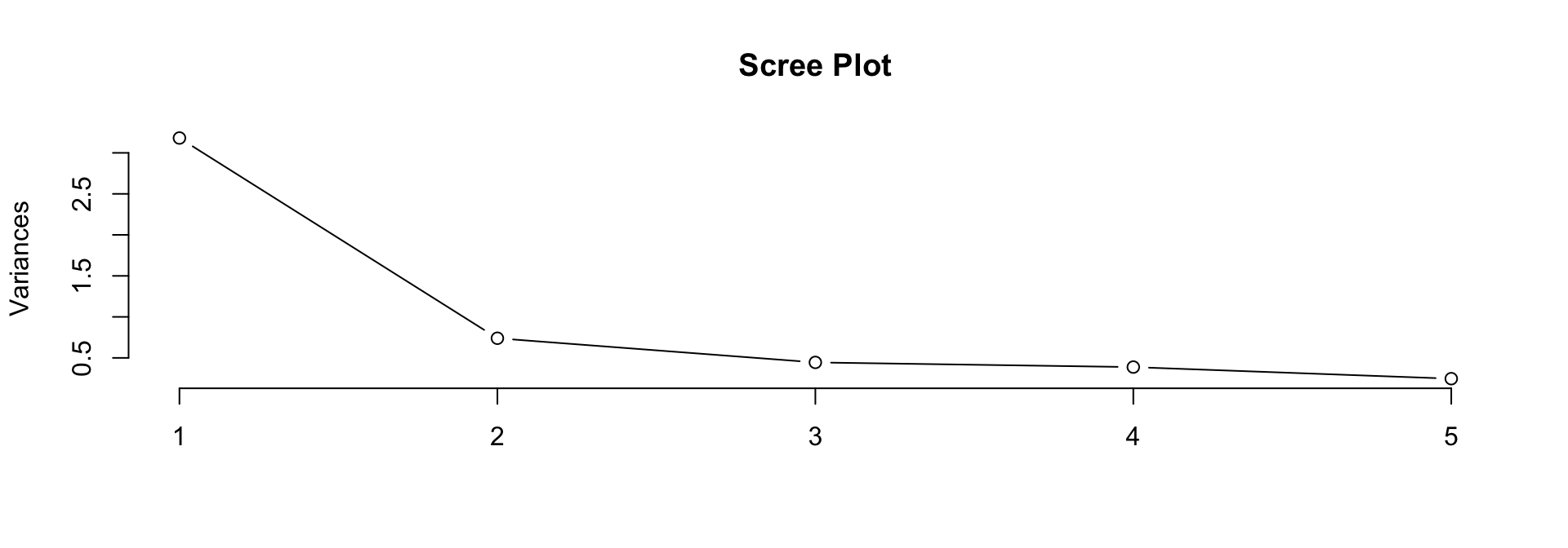
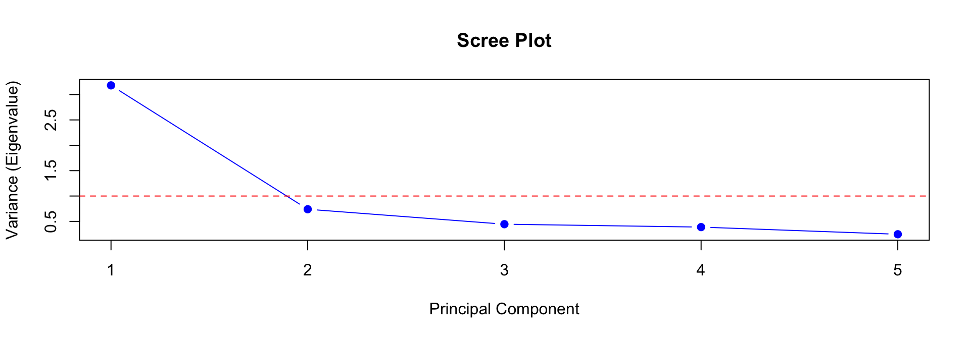
“Elbow” appears around PC2-3 → suggests keeping 2-3 components

Cumulative Variance Plot

Another way to decide how many components to keep:

plot(1:5, cumsum(prop_var), type = "b",
     xlab = "Number of Components",
     ylab = "Cumulative Proportion of Variance",
     main = "Cumulative Variance Explained",
     pch = 19, col = "darkgreen", ylim = c(0, 1))
abline(h = 0.8, lty = 2, col = "red")
abline(h = 0.9, lty = 2, col = "orange")
text(3, 0.82, "80% threshold", col = "red")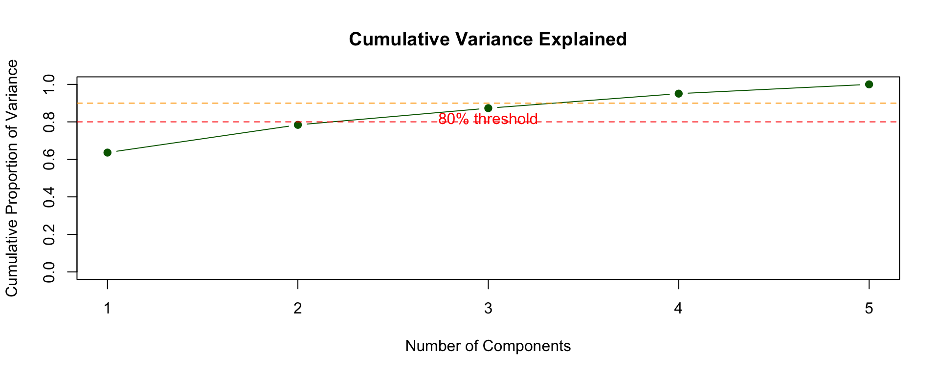

Rule of thumb: Keep enough PCs to explain 80-90% of variance

PC Scores: The Transformed Data

Scores are the actual PC values for each observation:

head(pca_result$x, 10)

         PC1         PC2        PC3         PC4         PC5
1  -4.285041 -0.67410225  0.1235891  0.79311084 -0.51438033
2  -4.541989  0.21331176 -0.2317797  0.55160634  0.59618974
3  -4.102690 -0.27557530  0.5304377  0.60968618 -0.02781595
4  -3.026846  0.14916207 -0.3702154  0.15958897 -0.43950477
5  -2.882081  0.04408014  0.2988861 -0.32257398 -0.14767795
6  -2.988775  0.68126196  0.2628756  0.29503310  0.54754485
7  -2.712178  0.35836879 -0.2052017  0.28351062 -0.03891465
8  -2.738431 -0.40679075 -0.2823520 -0.06940714  0.34696306
9  -2.360712  0.07851216  0.6488411  0.31562205 -0.52398228
10 -2.260005 -1.05560241 -0.3834319 -0.40401135 -0.20638713

These are the new coordinates in PC space:

Each student now represented by 5 PC scores instead of 5 exam scores
But the first 2-3 PCs contain most information!
PC1 = overall performance, PC2 = math type contrast

Visualizing PCs: Biplot

Biplot shows both observations and variable loadings:

biplot(pca_result, scale = 0, cex = 0.6)

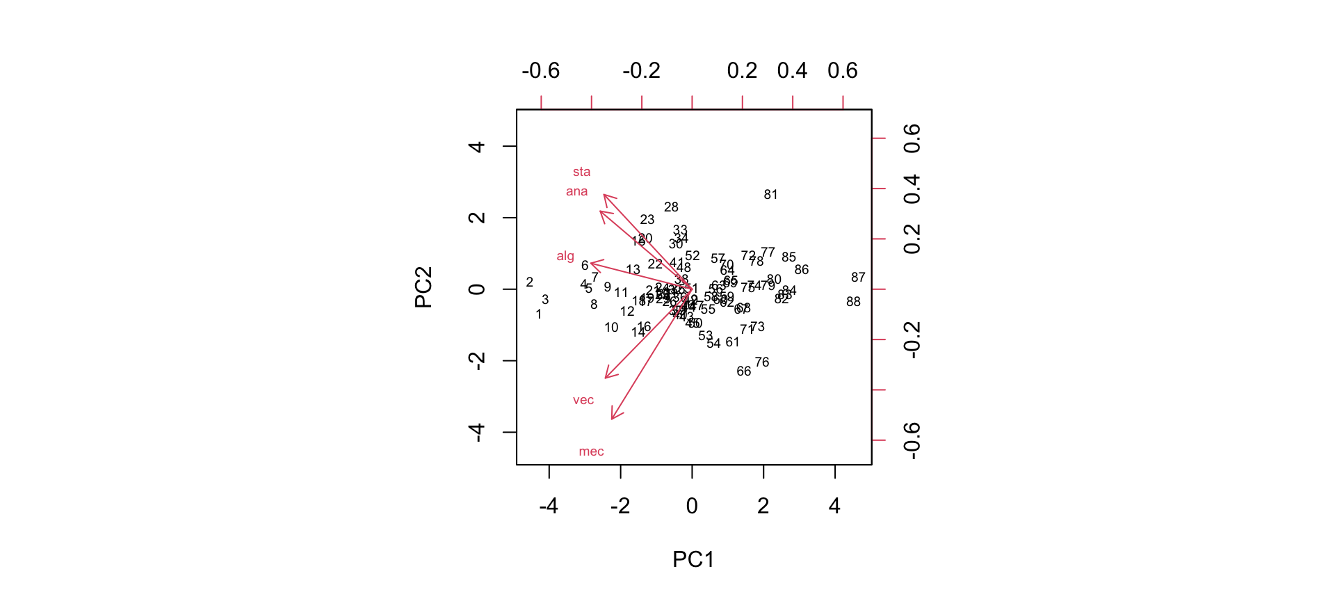
Reading the biplot:

Points = students in PC1-PC2 space
Arrows = original variables projected onto PCs
Arrow length = importance of variable
Arrow angle = correlation between variables

🎯 Activity: Interpret the Biplot

Pair Work (5 minutes):

Looking at the biplot:

Which exam scores are most similar (arrows point in same direction)?
Student 81 has high values on PC2. What does this tell you about their exam performance?
Students 87-88 are on the far right. What characterizes them?
Which exam appears most different from the others?

Hint:

Arrows pointing same direction = positively correlated
Arrow length = how well represented in 2D space
Position along PC1 = overall performance
Position along PC2 = math type

Discuss with your partner, then we’ll share on Ed Discussion.

Choosing Number of Components

Several criteria exist:

1. Kaiser Criterion (Eigenvalue > 1)

Keep PCs with eigenvalue > 1
Only for correlation matrix (standardized)
For us: Keep PC1 and PC2 (λ₁=3.18, λ₂=0.74… wait, only PC1!)

2. Proportion of Variance

Keep enough PCs to explain 80-90% variance
For us: 2 PCs explain 78%, 3 PCs explain 87%

Choosing Number of Components

Several criteria exist:

3. Scree Plot Elbow

Look for “elbow” where variance drops off
For us: Elbow suggests 2-3 components

4. Context-specific

What’s the purpose? Visualization? Prediction?
For visualization: usually keep 2-3 PCs

Standardization: Why It Matters

Let’s see the difference:

# PCA without scaling
pca_no_scale <- prcomp(scor, scale = FALSE)

# PCA with scaling  
pca_scaled <- prcomp(scor, scale = TRUE)

# Compare variance explained
data.frame(
  PC = 1:5,
  Unscaled = round(pca_no_scale$sdev^2 / sum(pca_no_scale$sdev^2), 3),
  Scaled = round(pca_scaled$sdev^2 / sum(pca_scaled$sdev^2), 3)
)

  PC Unscaled Scaled
1  1    0.619  0.636
2  2    0.182  0.148
3  3    0.093  0.089
4  4    0.076  0.078
5  5    0.029  0.049

Recommendation: Always use scale = TRUE unless variables already in same units!

Reconstructing Data from PCs

We can approximate original data using fewer PCs:

# Original data (scaled)
X_scaled <- scale(scor)

# Use only first 2 PCs to reconstruct
PC_scores_2 <- pca_result$x[, 1:2]
loadings_2 <- pca_result$rotation[, 1:2]
X_reconstructed <- PC_scores_2 %*% t(loadings_2)

# Compare original vs reconstructed for student 1
rbind(
  Original = X_scaled[1, ],
  Reconstructed = X_reconstructed[1, ],
  Difference = X_scaled[1, ] - X_reconstructed[1, ]
)

                     mec       vec       alg       ana       sta
Original      2.17573873 2.3890787  1.543347  1.368669 2.2423565
Reconstructed 2.14742649 2.1462680  2.069577  1.696749 1.5607605
Difference    0.02831224 0.2428107 -0.526230 -0.328080 0.6815959

With 2 PCs, we capture most structure but lose some detail

Visualizing in PC Space

Plot students in the reduced 2D space:

plot(pca_result$x[, 1], pca_result$x[, 2],
     xlab = "PC1 (63.6% variance)", 
     ylab = "PC2 (14.8% variance)",
     main = "Students in Principal Component Space",
     pch = 19, col = "steelblue")
text(pca_result$x[, 1], pca_result$x[, 2], 
     labels = 1:nrow(scor), pos = 3, cex = 0.6)
abline(h = 0, v = 0, lty = 2, col = "gray")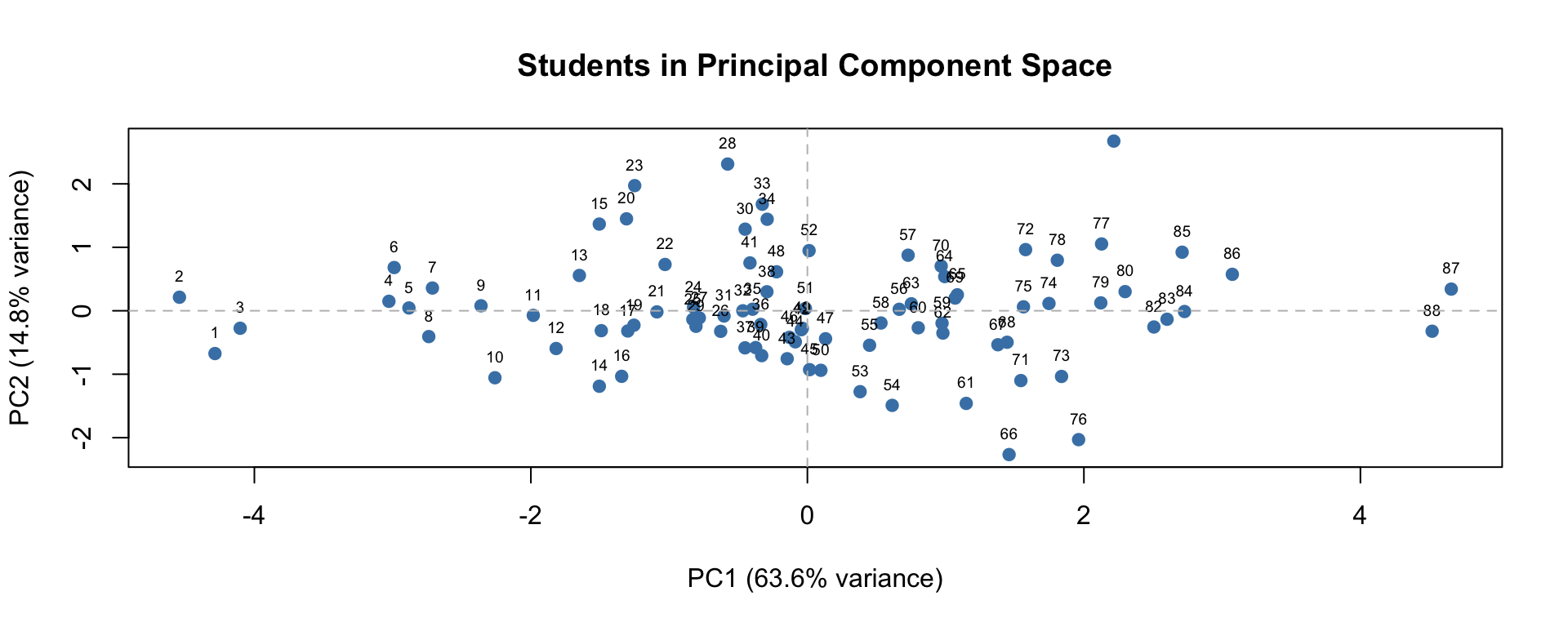

Now we can see student clustering patterns in 2D!

🎯 Activity: Perform Your Own PCA

Individual Work (8 minutes):

# Built-in mtcars dataset: car specifications
data(mtcars)
head(mtcars)

# Your tasks:
# 1. Examine correlations between variables
cor(mtcars)

# 2. Perform PCA with scaling
pca_cars <- prcomp(mtcars, scale = TRUE)

# 3. How much variance do first 2 PCs explain?


# 4. Look at PC1 loadings - what does PC1 represent?
pca_cars$rotation[, 1]

# 5. Make a biplot
biplot(pca_cars, scale = 0)

# 6. Create scree plot and decide how many PCs to keep


# Questions to answer:
# - What does PC1 seem to measure? (hint: look at loadings)
# - How many PCs would you keep and why?
# - Which variables are most correlated with PC1?

Post your findings on Ed Discussion!

PCA in Practice: MNIST Digits

Real application: Handwritten digit recognition

Each image = 784 pixels (28×28). Can we reduce this?

From your reference slides:

784 dimensions reduced to 50
Still can distinguish digits!
~90% variance retained with 100 PCs
First PC often captures “average digit” shape
Subsequent PCs capture variations

Common Applications of PCA

1. Dimensionality Reduction

Reduce 10,000 gene expressions → 50 PCs for analysis
Makes computation feasible

2. Visualization

Plot first 2-3 PCs to see clusters/patterns
Impossible to visualize 100+ dimensions directly

3. Dealing with Multicollinearity

Use PCs as predictors in regression instead of original variables
PCs are uncorrelated by construction

Common Applications of PCA

4. Data Compression

Store data more efficiently
Image/signal processing

5. Feature Engineering

Create new features for machine learning
Sometimes PCs are better predictors than raw variables

Principal Component Regression

Problem: Multicollinearity in predictors → unstable regression

Solution: Use PC scores as predictors instead!

# Regular regression (might have multicollinearity)
model_original <- lm(mpg ~ cyl + disp + hp + wt + qsec, 
                     data = mtcars)

# Extract PC scores
pca_cars <- prcomp(mtcars[, -1], scale = TRUE)
pc_scores <- pca_cars$x[, 1:3]  # Keep first 3 PCs

# Regression on PCs (no multicollinearity!)
model_pc <- lm(mtcars$mpg ~ pc_scores)

# PCs are uncorrelated by definition
cor(pc_scores)

Benefits:

No multicollinearity
Often better prediction with fewer variables
More stable coefficient estimates

Limitations and Assumptions of PCA

PCA assumes:

Linear relationships between variables
- PCA finds linear combinations
- May miss nonlinear patterns
Variance = information
- Assumes directions of high variance are important
- Sometimes low-variance directions matter!
Interpretation challenges
- PCs are combinations of all variables
- Can be hard to interpret meaningfully

Limitations and Assumptions of PCA

Sensitive to outliers
- Outliers can dominate PC directions
- Consider robust PCA alternatives

When PCA may not work well:

Categorical variables (use correspondence analysis instead)
Very sparse data
When you need interpretable original variables

What PCA Does NOT Do

❌ PCA Does NOT:

Automatically select “best” variables
Perform feature selection
Handle categorical variables well
Tell you causal relationships
Guarantee interpretable components
Always improve prediction

✓ PCA DOES:

Create uncorrelated combinations
Preserve total variance
Reduce dimensionality
Help with multicollinearity
Enable visualization
Reveal correlation structure

Remember: PCA is unsupervised - doesn’t use response variable!

Best Practices for PCA

Before running PCA:

Examine your data
- Check for outliers
- Look at variable distributions
- Understand the correlation structure
Decide on scaling
- Different units? → scale = TRUE
- Want variables weighted by variance? → scale = FALSE

Best Practices for PCA

During PCA:

Check variance explained
- Make informed decision about how many PCs
- Consider your goal (visualization vs prediction vs compression)

After PCA:

Interpret carefully
- Look at loadings to understand what PCs represent
- Use biplots to visualize
- Remember: interpretation is somewhat subjective!

Complete R Workflow

# Step 1: Load and explore data
data(scor, package = "bootstrap")
summary(scor)
cor(scor)

# Step 2: Perform PCA
pca <- prcomp(scor, scale = TRUE)

# Step 3: Examine variance explained
summary(pca)
screeplot(pca, type = "lines")

# Step 4: Look at loadings
pca$rotation[, 1:3]

# Step 5: Visualize
biplot(pca, scale = 0)

# Step 6: Use PC scores if needed
pc_scores <- pca$x[, 1:2]  # Keep first 2
head(pc_scores)

# Step 7: Extract variance proportions
pca_var <- pca$sdev^2
pve <- pca_var / sum(pca_var)
cumsum(pve)

Student Practice (10 minutes)

Your Turn: Comprehensive PCA Analysis

# Use the USArrests dataset
data(USArrests)
?USArrests  # Read about the data

# Your tasks:
# 1. Explore the data
head(USArrests)
summary(USArrests)
pairs(USArrests)  # Scatterplot matrix

# 2. Calculate and visualize correlations


# 3. Perform PCA (with scaling - why is this important here?)


# 4. Answer these questions:
#    a) How many PCs would you retain and why?
#    b) What does PC1 represent? Interpret the loadings.
#    c) What does PC2 represent?
#    d) Which states have highest PC1 scores? Lowest?
#    e) Make a biplot - which variables are most correlated?

# 5. Create all relevant visualizations:
#    - Scree plot
#    - Cumulative variance plot  
#    - Biplot
#    - PC1 vs PC2 scatter with state labels

# 6. Reconstruct data using only 2 PCs
#    How much information did we lose?

Common Mistakes to Avoid

❌ Don’t:

Forget to scale when variables have different units
Keep too few PCs (losing important information)
Over-interpret small loadings
Ignore the scree plot
Use PCA on categorical data
Assume PCs are always interpretable

✓ Do:

Always check if scaling is needed
Use multiple criteria for # of PCs
Focus on large (absolute) loadings
Create visualizations
Check correlation structure first
Remember PCA is exploratory

Most important: Understand your data and your goal before applying PCA!

Connection to Other Methods

PCA is related to many other techniques:

Factor Analysis

Similar to PCA but different goals
FA assumes latent factors cause observed variables
PCA just summarizes variance

Correspondence Analysis

PCA for categorical data
Used in text mining, surveys

Connection to Other Methods

Singular Value Decomposition (SVD)

PCA is special case of SVD
SVD works on data matrix directly

Multidimensional Scaling (MDS)

Preserves distances between observations
PCA is a special case (when using Euclidean distance)

Summary

PCA reduces dimensionality by creating uncorrelated linear combinations
Based on eigendecomposition of covariance/correlation matrix
PC1 captures most variance, PC2 second most, etc.
Loadings show how original variables combine to create PCs
Scores are the actual PC values for each observation
Use scree plots and cumulative variance to decide how many PCs to keep
Scaling is crucial when variables have different units
PCA reveals correlation structure in your data

When to use PCA:

Too many correlated variables
Need to visualize high-dimensional data
Want to deal with multicollinearity
Data compression

Quick Reference: Key Functions

# Perform PCA
pca <- prcomp(data, scale = TRUE)

# Variance explained
summary(pca)
pca$sdev^2  # Eigenvalues

# Loadings
pca$rotation

# Scores
pca$x

# Visualizations
screeplot(pca, type = "lines")
biplot(pca, scale = 0)

# Variance proportions
prop_var <- pca$sdev^2 / sum(pca$sdev^2)
cumsum(prop_var)

# Correlation plot (before PCA)
library(corrplot)
corrplot(cor(data))

Final Questions & Next Steps

For next class:

Clusters

Office Hours: After class today

🗓️ Week 07 Principal Component Analysis (PCA)

Class Overview

Motivation: The Curse of Dimensionality

Why Do We Need PCA?

Why Do We Need PCA?

What Exactly Does PCA Do?

Our Running Example: Test Scores

Exploring Correlations

The Mathematics Behind PCA

Covariance vs. Correlation Matrix

Performing PCA in R

Understanding PC Loadings

Interpreting PC2

Variance Explained by Each PC

Visualizing Variance Explained: Scree Plot

Cumulative Variance Plot

PC Scores: The Transformed Data

Visualizing PCs: Biplot

🎯 Activity: Interpret the Biplot

Choosing Number of Components

Choosing Number of Components

Standardization: Why It Matters

Reconstructing Data from PCs

Visualizing in PC Space

🎯 Activity: Perform Your Own PCA

PCA in Practice: MNIST Digits

Common Applications of PCA

Common Applications of PCA

Principal Component Regression

Limitations and Assumptions of PCA

Limitations and Assumptions of PCA

What PCA Does NOT Do

❌ PCA Does NOT:

✓ PCA DOES:

Best Practices for PCA

Best Practices for PCA

Complete R Workflow

Student Practice (10 minutes)

Common Mistakes to Avoid

❌ Don’t:

✓ Do:

Connection to Other Methods

Connection to Other Methods

Summary

Quick Reference: Key Functions

Final Questions & Next Steps

🗓️ Week 07
Principal Component Analysis (PCA)