[1] "Log-odds: 1"[1] "Odds: 2.718"[1] "Probability: 0.731"STAT 204 – Introduction to Statistical Data Analysis
04 Nov 2025
Today’s Focus:
Learning Goals: Understand the theory and practice of modeling binary outcomes
Linear regression works great for continuous outcomes:
But what about binary outcomes?
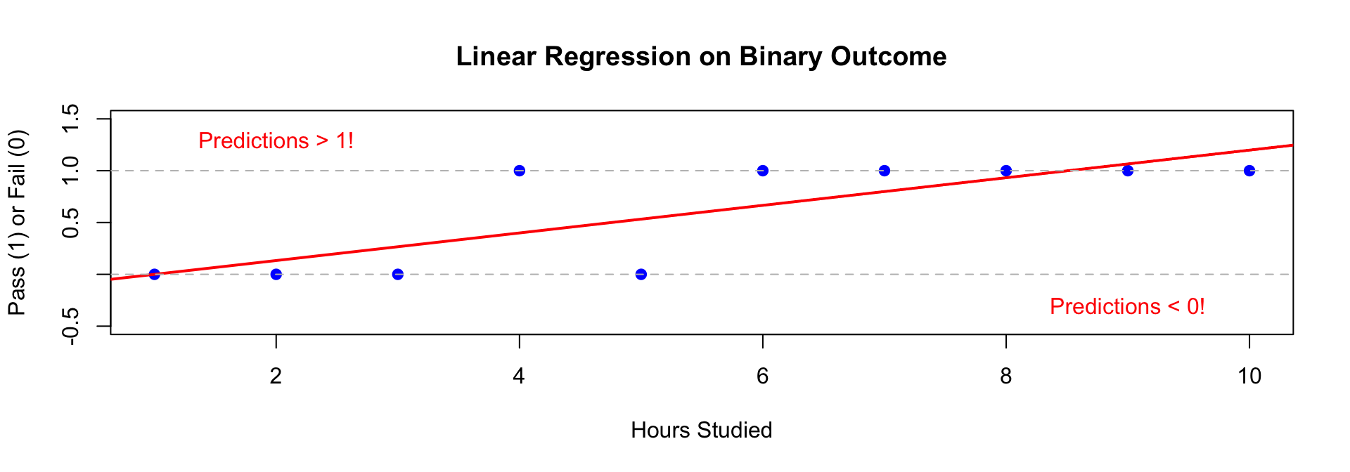
Problem: Linear regression predicts values outside [0,1]!
Example: Predict exam pass (1) or fail (0) from hours studied
Problems:
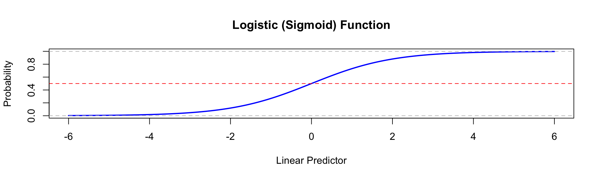
We need a transformation that maps (-∞, ∞) to (0, 1)
The sigmoid function (logistic function) does exactly this:
\[p(x) = \frac{1}{1 + e^{-(\beta_0 + \beta_1 x)}}\]
Probability: \(p = P(Y=1)\)
Odds: \(\frac{p}{1-p} = \frac{P(Y=1)}{P(Y=0)}\)
Examples:
Log-odds (logit): \(\log\left(\frac{p}{1-p}\right)\)
This is our linear predictor!
The model links linear predictors to probability:
\[\log\left(\frac{p}{1-p}\right) = \beta_0 + \beta_1 x_1 + \beta_2 x_2 + \cdots + \beta_p x_p\]
Or equivalently:
\[p = \frac{1}{1 + e^{-(\beta_0 + \beta_1 x_1 + \cdots + \beta_p x_p)}}\]
Key differences from linear regression:
For each observation: \(Y_i \sim \text{Bernoulli}(p_i)\)
Likelihood for observation i: \[L_i = p_i^{y_i}(1-p_i)^{1-y_i}\]
Why this works:
Total likelihood (assuming independence): \[L(\beta) = \prod_{i=1}^n p_i^{y_i}(1-p_i)^{1-y_i}\]
Log-likelihood (easier to work with): \[\ell(\beta) = \sum_{i=1}^n [y_i \log(p_i) + (1-y_i)\log(1-p_i)]\]
Substitute \(p_i = \frac{1}{1 + e^{-X_i\beta}}\):
\[\ell(\beta) = \sum_{i=1}^n \left[y_i(X_i\beta) - \log(1 + e^{X_i\beta})\right]\]
Goal: Find \(\hat{\beta}\) that maximizes \(\ell(\beta)\)
Problem: No closed-form solution! (Unlike OLS)
In OLS: Taking derivative and setting to zero gives: \[\hat{\beta}_{OLS} = (X'X)^{-1}X'y\]
In Logistic Regression: The score equation is: \[\frac{\partial \ell}{\partial \beta} = \sum_{i=1}^n X_i(y_i - p_i) = 0\]
But \(p_i\) depends on \(\beta\) nonlinearly: \[p_i = \frac{1}{1 + e^{-X_i\beta}}\]
This creates a nonlinear system with no closed-form solution.
Solution: Use iterative methods!
Newton-Raphson Algorithm:
Alternatively: IRLS (Iteratively Reweighted Least Squares)
In R: glm() uses IRLS by default
Under regularity conditions, MLEs are:
Consistent: \(\hat{\beta} \xrightarrow{p} \beta\) as \(n \to \infty\)
Asymptotically normal: \[\sqrt{n}(\hat{\beta} - \beta) \xrightarrow{d} N(0, I(\beta)^{-1})\]
where \(I(\beta)\) is the Fisher Information matrix
Asymptotically efficient: Lowest variance among consistent estimators
Invariant: If \(\hat{\beta}\) maximizes \(\ell\), then \(g(\hat{\beta})\) maximizes likelihood of \(g(\beta)\)
Practical implications:
Given: \(\log\left(\frac{p}{1-p}\right) = -2 + 0.5 \times \text{StudyHours}\)
For a student who studied 6 hours:
[1] "Log-odds: 1"[1] "Odds: 2.718"[1] "Probability: 0.731"Interpretation: Student has 73.1% chance of passing.
Remember: Coefficients represent change in log-odds, not probability!
For a one-unit increase in \(x_j\):
Example: \(\beta_1 = 0.3\) for years of education
Unlike linear regression: Effect on probability depends on starting point!
[1] "Odds Ratio: 1.35"[1] "Odds multiply by 1.35"[1] "Percent increase: 35 %"Confidence intervals for odds ratios: \[\exp(\beta \pm 1.96 \times SE(\beta))\]
Pair Work (6 minutes):
Coefficients:
                Estimate Std. Error z value Pr(>|z|)
(Intercept)     -4.2100     0.8200  -5.134  < 0.001 ***
age              0.0450     0.0150   3.000  0.00270 **
income           0.0002     0.0001   2.000  0.04550 *
education        0.3200     0.1200   2.667  0.00766 **
Tasks:
education (response variable is employed yes/no)Discuss your answers with your partner, then we’ll share them on Ed Discussion.
In linear regression: R² measures proportion of variance explained
Problem for binary outcomes:
Alternative approaches:
Classify predictions using a threshold (usually 0.5)
| Predicted: No | Predicted: Yes | |
|---|---|---|
| Actual: No | True Negative (TN) | False Positive (FP) |
| Actual: Yes | False Negative (FN) | True Positive (TP) |
Key metrics:
Question: Which predictors should we include in our logistic model?
Same challenge as linear regression:
Solution: Cross-validation!
Algorithm:
Metrics to track:
library(caret)
library(titanic)
data(titanic_train)

# Remove missing values
titanic <- na.omit(titanic_train)

# Convert Survived to factor with proper names
# 0 = "Died", 1 = "Survived" (or any valid R names)
titanic$Survived_factor <- factor(titanic$Survived,
                                  levels = c(0, 1),
                                  labels = c("Died", "Survived"))

# Set up 10-fold cross-validation
train_control <- trainControl(
  method = "cv",
  number = 10,
  summaryFunction = twoClassSummary,  # For ROC, Sens, Spec
  classProbs = TRUE,                   # Needed for ROC
  savePredictions = TRUE
)

# Fit model with CV (use Survived_factor, not Survived)
model_cv <- train(
  Survived_factor ~ Pclass + Sex + Age + Fare,
  data = titanic,
  method = "glm",
  family = "binomial",
  trControl = train_control,
  metric = "ROC"  # Optimize for AUC
)

# View results
print(model_cv)
model_cv$results# Model 1: Simple
model1_cv <- train(
Survived_factor ~ Pclass + Sex + Age,
data = titanic,
method = "glm",
family = "binomial",
trControl = train_control,
metric = "ROC"
)
# Model 2: More complex
model2_cv <- train(
Survived_factor ~ Pclass + Sex + Age + Fare + SibSp + Parch,
data = titanic,
method = "glm",
family = "binomial",
trControl = train_control,
metric = "ROC"
)
# Compare results
results <- resamples(list(Simple = model1_cv, Complex = model2_cv))
summary(results)
bwplot(results) # Boxplot of performance across foldsAlternative to CV: Use information criteria for quick model comparison
AIC (Akaike Information Criterion): \[\text{AIC} = -2\ell(\hat{\beta}) + 2p\]
BIC (Bayesian Information Criterion): \[\text{BIC} = -2\ell(\hat{\beta}) + p\log(n)\]
where:
Lower is better! BIC penalizes complexity more than AIC.
# Fit several models
model1 <- glm(Survived_factor ~ Pclass + Sex,
              data = titanic, family = binomial)
model2 <- glm(Survived_factor ~ Pclass + Sex + Age,
              data = titanic, family = binomial)
model3 <- glm(Survived_factor ~ Pclass + Sex + Age + Fare + SibSp,
              data = titanic, family = binomial)

# Compare AIC
AIC(model1, model2, model3)

# Compare BIC
BIC(model1, model2, model3)

# Stepwise selection using AIC
library(MASS)
full_model <- glm(Survived_factor ~ Pclass + Sex + Age + Fare + SibSp + Parch,
                  data = titanic, family = binomial)
step_model <- stepAIC(full_model, direction = "both", trace = FALSE)
summary(step_model)Pair Work (8 minutes):
library(caret)
library(titanic)
data(titanic_train)
titanic <- na.omit(titanic_train)

# IMPORTANT: Convert to factor with valid names
titanic$Survived_factor <- factor(titanic$Survived,
                                  levels = c(0, 1),
                                  labels = c("Died", "Survived"))

# Your task: Compare at least 3 different models

# Set up CV
train_control <- trainControl(
  method = "cv", number = 10,
  summaryFunction = twoClassSummary,
  classProbs = TRUE
)

# Model A: Your choice (use Survived_factor)
modelA <- train(Survived_factor ~ ..., data = titanic,
                method = "glm", family = "binomial",
                trControl = train_control, metric = "ROC")

# Model B: Your choice
modelB <- train(Survived_factor ~ ..., data = titanic,
                method = "glm", family = "binomial",
                trControl = train_control, metric = "ROC")

# Model C: Your choice
modelC <- train(Survived_factor ~ ..., data = titanic,
                method = "glm", family = "binomial",
                trControl = train_control, metric = "ROC")

# Compare
results <- resamples(list(A = modelA, B = modelB, C = modelC))
summary(results)
Questions: Which model has highest AUC? Does it match AIC/BIC?
ROC (Receiver Operating Characteristic) Curve:
AUC (Area Under the Curve):
Use ROC/AUC when:
Default: 0.5 — but not always optimal!
Considerations:
Methods:
Live Coding Demo: Titanic Survival
# Load data
library(titanic)
data(titanic_train)
titanic <- titanic_train

# Explore
head(titanic)
table(titanic$Survived)

# Fit logistic regression
model <- glm(Survived ~ Pclass + Sex + Age + SibSp + Parch + Fare,
             data = titanic,
             family = binomial(link = 'logit'))

# View results
summary(model)

# Odds ratios
exp(coef(model))
exp(confint(model))

# Predictions (probabilities)
titanic$pred_prob <- predict(model, type = 'response')

# Classify with threshold 0.5
titanic$pred_class <- ifelse(titanic$pred_prob > 0.5, 1, 0)

# Confusion matrix
table(Actual = titanic$Survived, Predicted = titanic$pred_class)

# Calculate metrics
library(caret)
confusionMatrix(factor(titanic$pred_class),
                factor(titanic$Survived),
                positive = "1")

# ROC curve
library(pROC)
roc_obj <- roc(titanic$Survived, titanic$pred_prob)
plot(roc_obj, main = paste("AUC =", round(auc(roc_obj), 3)))
auc(roc_obj)Your Turn:
library(titanic)
library(caret)
data(titanic_train)
titanic <- na.omit(titanic_train)

# For caret: Convert to factor with valid names
titanic$Survived_factor <- factor(titanic$Survived,
                                  levels = c(0, 1),
                                  labels = c("Died", "Survived"))

# 1. Fit a logistic regression model with your chosen predictors
your_model <- glm(Survived_factor ~ ...,  # glm() is fine with 0/1
                  data = titanic,
                  family = binomial)

# 2. Examine coefficients and calculate odds ratios
summary(your_model)
exp(coef(your_model))
exp(confint(your_model))

# 3. Compare with stepwise selection
library(MASS)
full_model <- glm(Survived_factor ~ Pclass + Sex + Age + Fare + SibSp + Parch, data = titanic, family = binomial)
step_model <- stepAIC(full_model, direction = "both")

# 4. Generate predictions
pred_probs <- predict(your_model, type = 'response')

# 5. Create confusion matrix (threshold = 0.5)
pred_class <- ifelse(pred_probs > 0.5, 1, 0)
table(Actual = titanic$Survived_factor, Predicted = pred_class)

# 6. Calculate metrics and ROC/AUC
library(caret)
confusionMatrix(factor(pred_class), factor(titanic$Survived),
                positive = "1")

library(pROC)
roc_result <- roc(titanic$Survived_factor, pred_probs)
plot(roc_result)
auc(roc_result)

# 7. Use cross-validation to compare models
# IMPORTANT: Use Survived_factor for caret!
train_control <- trainControl(method = "cv", number = 10,
                              summaryFunction = twoClassSummary,
                              classProbs = TRUE)
cv_model <- train(Survived_factor ~ ..., data = titanic,
                  method = "glm", family = "binomial",
                  trControl = train_control, metric = "ROC")
print(cv_model)Problem: 95% negative, 5% positive → model predicts all negative, gets 95% accuracy!
Solutions:
| Feature | Linear Regression | Logistic Regression |
|---|---|---|
| Outcome | Continuous | Binary (0/1) |
| Distribution | Normal | Bernoulli |
| Link function | Identity | Logit |
| Interpretation | Direct effect on Y | Effect on log-odds |
| Estimation | OLS (closed-form) | MLE (iterative) |
| Predictions | Any real number | Probability [0,1] |
| Evaluation | R², RMSE | Accuracy, AUC, sensitivity |
Key Takeaways:
Connection to what you know:
For next class:
Office Hours: After class today

STAT 204 – Intro to Statistical Data Analysis