🗓️ Week 05
Model Selection & ANOVA

STAT 204 – Introduction to Statistical Data Analysis

Prof. Marcela Alfaro Cordoba

Statistics - UCSC

28 Oct 2025

Part 1: Model Selection & Information Criteria

Class Overview - Part 1

Today’s Focus:

The model selection problem
Bias-variance tradeoff
Stepwise selection methods
Information criteria (AIC/BIC)
Cross-validation basics

Learning Goals: Understand when and how to select the best predictive model

Model Selection: The Problem

We often have many potential predictors. Questions:

Which predictors should we include?
Is a more complex model better? - Description vs Prediction
How do we balance fit vs. complexity?

Goal for Prediction: Find the model that predicts best on new data!

Bias-Variance Tradeoff

Underfitting (too simple):

High bias, low variance
Poor fit to training and test data

Overfitting (too complex):

Low bias, high variance
Great fit to training data, poor on test data

Goal: Find the sweet spot!

🎯 Activity 1: Visualizing Overfitting

Work in pairs:

# Generate data with a simple relationship
set.seed(123)
x <- seq(0, 10, length.out = 20)
y <- 2 + 3*x + rnorm(20, sd = 5)

# Fit models of increasing complexity
model1 <- lm(y ~ x)
model2 <- lm(y ~ poly(x, 3))
model3 <- lm(y ~ poly(x, 10))

# Plot and compare
par(mfrow=c(1,3))
plot(x, y, main="Linear (Simple)")
abline(model1, col="red", lwd=2)

plot(x, y, main="Cubic (Moderate)")
lines(sort(x), fitted(model2)[order(x)], col="blue", lwd=2)

plot(x, y, main="10th degree (Complex)")
lines(sort(x), fitted(model3)[order(x)], col="green", lwd=2)

Discuss: Which model would you choose and why?

Model Selection Strategies

All subsets regression: Try all possible models (computationally expensive)
Stepwise regression: Add/remove predictors sequentially
Information criteria: AIC, BIC
Cross-validation: Estimate prediction error directly
Regularization: Penalize complexity (LASSO, Ridge) - next course!

Forward Selection

Algorithm:

Start with intercept-only model
Add predictor that improves model most
Repeat until no improvement
Stop based on criterion (AIC, p-value, etc.)

library(MASS)
library(palmerpenguins)
library(dplyr)

# Forward selection using AIC
step(lm(body_mass_g ~ 1, data = penguins),
     scope = ~ flipper_length_mm + bill_length_mm + bill_depth_mm + species,
     direction = "forward")

Start:  AIC=4574.94
body_mass_g ~ 1

                    Df Sum of Sq       RSS    AIC
+ flipper_length_mm  1 166452902  52854796 4090.3
+ species            2 146864214  72443483 4200.1
+ bill_length_mm     1  77669072 141638626 4427.4
+ bill_depth_mm      1  48840779 170466918 4490.8
<none>                           219307697 4574.9

Step:  AIC=4090.3
body_mass_g ~ flipper_length_mm

                 Df Sum of Sq      RSS    AIC
+ species         2   5187807 47666988 4059.0
+ bill_depth_mm   1    449044 52405752 4089.4
<none>                        52854796 4090.3
+ bill_length_mm  1    211671 52643125 4090.9

Step:  AIC=4058.97
body_mass_g ~ flipper_length_mm + species

                 Df Sum of Sq      RSS    AIC
+ bill_depth_mm   1  10796029 36870959 3973.1
+ bill_length_mm  1   8683628 38983360 3992.2
<none>                        47666988 4059.0

Step:  AIC=3973.14
body_mass_g ~ flipper_length_mm + species + bill_depth_mm

                 Df Sum of Sq      RSS    AIC
+ bill_length_mm  1   3344286 33526673 3942.6
<none>                        36870959 3973.1

Step:  AIC=3942.62
body_mass_g ~ flipper_length_mm + species + bill_depth_mm + bill_length_mm


Call:
lm(formula = body_mass_g ~ flipper_length_mm + species + bill_depth_mm + 
    bill_length_mm, data = penguins)

Coefficients:
      (Intercept)  flipper_length_mm   speciesChinstrap      speciesGentoo  
         -4327.33              20.24            -513.25             934.89  
    bill_depth_mm     bill_length_mm  
           140.33              41.47

Backward Selection

Algorithm:

Start with full model (all predictors)
Remove predictor that hurts model least
Repeat until no improvement
Stop based on criterion

# Backward selection using AIC
full_model <- lm(body_mass_g ~ flipper_length_mm + bill_length_mm + 
                   bill_depth_mm + species, 
                 data = penguins)

step(full_model, direction = "backward")

Start:  AIC=3942.62
body_mass_g ~ flipper_length_mm + bill_length_mm + bill_depth_mm + 
    species

                    Df Sum of Sq      RSS    AIC
<none>                           33526673 3942.6
- bill_length_mm     1   3344286 36870959 3973.1
- flipper_length_mm  1   4239352 37766025 3981.3
- bill_depth_mm      1   5456687 38983360 3992.2
- species            2  18784686 52311359 4090.8


Call:
lm(formula = body_mass_g ~ flipper_length_mm + bill_length_mm + 
    bill_depth_mm + species, data = penguins)

Coefficients:
      (Intercept)  flipper_length_mm     bill_length_mm      bill_depth_mm  
         -4327.33              20.24              41.47             140.33  
 speciesChinstrap      speciesGentoo  
          -513.25             934.89

Stepwise Selection

Combines forward and backward:

At each step, can add or remove a predictor
More flexible than pure forward or backward

# Stepwise selection
step(full_model, direction = "both")

Start:  AIC=3942.62
body_mass_g ~ flipper_length_mm + bill_length_mm + bill_depth_mm + 
    species

                    Df Sum of Sq      RSS    AIC
<none>                           33526673 3942.6
- bill_length_mm     1   3344286 36870959 3973.1
- flipper_length_mm  1   4239352 37766025 3981.3
- bill_depth_mm      1   5456687 38983360 3992.2
- species            2  18784686 52311359 4090.8


Call:
lm(formula = body_mass_g ~ flipper_length_mm + bill_length_mm + 
    bill_depth_mm + species, data = penguins)

Coefficients:
      (Intercept)  flipper_length_mm     bill_length_mm      bill_depth_mm  
         -4327.33              20.24              41.47             140.33  
 speciesChinstrap      speciesGentoo  
          -513.25             934.89

🎯 Activity 2: Compare Selection Methods

Group Exercise:

# Create a full model with all available predictors
full_model <- lm(body_mass_g ~ flipper_length_mm + bill_length_mm + 
                   bill_depth_mm + species + sex + island, 
                 data = penguins)

# Try different directions
step_forward <- step(lm(body_mass_g ~ 1, data = penguins),
                     scope = formula(full_model),
                     direction = "forward", trace = 0)

step_backward <- step(full_model, direction = "backward", trace = 0)

step_both <- step(full_model, direction = "both", trace = 0)

# Compare the final models
summary(step_forward)$coefficients
summary(step_backward)$coefficients
summary(step_both)$coefficients

Questions to discuss:

Do all methods give the same final model?
If different, which variables differ?
Which method would you trust most?

Akaike Information Criterion (AIC)

AIC balances model fit and complexity:

\[\text{AIC} = -2\log(L) + 2p\]

where \(L\) is the likelihood and \(p\) is the number of parameters.

For linear regression: \[\text{AIC} = n\log(\text{SSR}/n) + 2p\]

Lower AIC is better! AIC penalizes adding parameters.

Bayesian Information Criterion (BIC)

BIC is similar to AIC but penalizes complexity more:

\[\text{BIC} = -2\log(L) + p\log(n)\]

For linear regression: \[\text{BIC} = n\log(\text{SSR}/n) + p\log(n)\]

Lower BIC is better! BIC tends to select simpler models than AIC.

Comparing Models with AIC/BIC

# Fit several models
model1 <- lm(body_mass_g ~ flipper_length_mm, data = penguins)
model2 <- lm(body_mass_g ~ flipper_length_mm + bill_length_mm, data = penguins)
model3 <- lm(body_mass_g ~ flipper_length_mm + bill_length_mm + species, 
             data = penguins)

# Compare AIC
AIC(model1, model2, model3)

       df      AIC
model1  3 5062.855
model2  4 5063.482
model3  6 4964.745

# Compare BIC
BIC(model1, model2, model3)

       df      BIC
model1  3 5074.359
model2  4 5078.822
model3  6 4987.754

Guideline: Difference in AIC > 2 suggests models are meaningfully different.

🎯 Activity 3: Build Your Best Model

Individual/Pair Work:

# Your task: Find the best model for predicting penguin body mass
# Available predictors: flipper_length_mm, bill_length_mm, 
#                       bill_depth_mm, species, sex, island

# Step 1: Fit at least 4 different models (your choice!)
model_a <- lm(body_mass_g ~ ..., data = penguins)
model_b <- lm(body_mass_g ~ ..., data = penguins)
model_c <- lm(body_mass_g ~ ..., data = penguins)
model_d <- lm(body_mass_g ~ ..., data = penguins)

# Step 2: Compare using AIC and BIC
AIC(model_a, model_b, model_c, model_d)
BIC(model_a, model_b, model_c, model_d)

# Step 3: Check diagnostics of your best model
plot(your_best_model)

# Step 4: Report your findings
summary(your_best_model)

Questions:

Which model has the lowest AIC? Lowest BIC?
Do AIC and BIC agree?
How much do the values differ?
Does your best model pass diagnostic checks?

Cross-Validation: The Gold Standard

Idea: Estimate prediction error on unseen data.

K-Fold Cross-Validation:

Split data into \(K\) folds
For each fold: train on \(K-1\) folds, test on remaining fold
Average the prediction errors

Common: \(K = 5\) or \(K = 10\)

Leave-One-Out Cross-Validation (LOOCV)

Special case: \(K = n\)

CV error: \[\text{CV} = \frac{1}{n}\sum_{i=1}^{n}(Y_i - \hat{Y}_{-i})^2\]

where \(\hat{Y}_{-i}\) is prediction for \(i\) using model trained without observation \(i\).

Computationally expensive but can use shortcut for linear regression!

LOOCV Shortcut for Linear Regression

\[\text{CV} = \frac{1}{n}\sum_{i=1}^{n}\left(\frac{e_i}{1 - h_{ii}}\right)^2\]

where \(e_i\) is the residual and \(h_{ii}\) is the leverage.

This is also called the PRESS statistic (Predicted Residual Sum of Squares).

Cross-Validation in R

# We'll use the caret package for easy CV implementation
# install.packages("caret") # if needed
library(caret)

# Set up 10-fold cross-validation
train_control <- trainControl(method = "cv", number = 10)

# Fit model with 10-fold CV
model_cv10 <- train(body_mass_g ~ flipper_length_mm + bill_length_mm + species,
                    data = penguins,
                    method = "lm",
                    trControl = train_control,
                    na.action = na.omit)

# View results
print(model_cv10)

Linear Regression 

344 samples
  3 predictor

No pre-processing
Resampling: Cross-Validated (10 fold) 
Summary of sample sizes: 308, 309, 309, 307, 308, 308, ... 
Resampling results:

  RMSE      Rsquared   MAE    
  340.0788  0.8275932  272.459

Tuning parameter 'intercept' was held constant at a value of TRUE

🎯 Activity 4: Cross-Validation

Group Exercise - Compare Different CV Methods:

Your task is to compare three models using different cross-validation approaches and determine which model predicts best!

library(caret)
library(palmerpenguins)

# Remove missing values first
penguins_clean <- na.omit(penguins[, c("body_mass_g", "flipper_length_mm", 
                                        "bill_length_mm", "bill_depth_mm", 
                                        "species", "sex")])

# Define three competing models
model_formulas <- list(
  simple = body_mass_g ~ flipper_length_mm,
  moderate = body_mass_g ~ flipper_length_mm + bill_length_mm + species,
  complex = body_mass_g ~ flipper_length_mm + bill_length_mm + 
                          bill_depth_mm + species + sex
)

# Function to perform CV with different K values
compare_cv_methods <- function(formula, data) {
  
  # 5-Fold CV
  ctrl_5fold <- trainControl(method = "cv", number = 5)
  cv5 <- train(formula, data = data, method = "lm", trControl = ctrl_5fold)
  
  # 10-Fold CV
  ctrl_10fold <- trainControl(method = "cv", number = 10)
  cv10 <- train(formula, data = data, method = "lm", trControl = ctrl_10fold)
  
  # Leave-One-Out CV (LOOCV)
  ctrl_loocv <- trainControl(method = "LOOCV")
  loocv <- train(formula, data = data, method = "lm", trControl = ctrl_loocv)
  
  # Return RMSE values
  return(data.frame(
    CV5_RMSE = cv5$results$RMSE,
    CV10_RMSE = cv10$results$RMSE,
    LOOCV_RMSE = loocv$results$RMSE,
    CV5_Rsquared = cv5$results$Rsquared,
    CV10_Rsquared = cv10$results$Rsquared,
    LOOCV_Rsquared = loocv$results$Rsquared
  ))
}

# Compare all three models
results_simple <- compare_cv_methods(model_formulas$simple, penguins_clean)
results_moderate <- compare_cv_methods(model_formulas$moderate, penguins_clean)
results_complex <- compare_cv_methods(model_formulas$complex, penguins_clean)

# Create comparison table
comparison <- data.frame(
  Model = c("Simple", "Moderate", "Complex"),
  rbind(results_simple, results_moderate, results_complex)
)

print(comparison)

# Visualize the results
## create a plot to visualize your results

Activity 4: Discussion Questions

After running the code, discuss:

Which model has the lowest prediction error (RMSE)?
- Does this match what AIC/BIC suggested?
How do the three CV methods (K=5, K=10, LOOCV) compare?
- Are the RMSE values similar or different?
- Which method took longest to run? Why?
What’s the trade-off between bias and variance?
- LOOCV has lower bias but higher variance
- K-fold has slightly higher bias but lower variance
Practical considerations:
- When would you use K=5 vs K=10 vs LOOCV?
- How does dataset size affect your choice?

Alternative: Manual K-Fold CV

For deeper understanding, implement CV manually:

# Manual 5-fold cross-validation
set.seed(123)
n <- nrow(penguins_clean)
K <- 5

# Create fold assignments
fold_ids <- sample(rep(1:K, length.out = n))

# Store predictions
cv_errors <- numeric(K)

for(k in 1:K) {
  # Split data
  test_idx <- which(fold_ids == k)
  train_data <- penguins_clean[-test_idx, ]
  test_data <- penguins_clean[test_idx, ]
  
  # Fit model on training data
  model <- lm(body_mass_g ~ flipper_length_mm + bill_length_mm + species, 
              data = train_data)
  
  # Predict on test data
  predictions <- predict(model, newdata = test_data)
  
  # Calculate MSE for this fold
  cv_errors[k] <- mean((test_data$body_mass_g - predictions)^2)
}

# Average across all folds
cv_mse <- mean(cv_errors)
cv_rmse <- sqrt(cv_mse)

cat("5-Fold CV RMSE:", round(cv_rmse, 2), "\n")
cat("Individual fold RMSEs:", round(sqrt(cv_errors), 2), "\n")

Activity 4: Extension Challenge (Optional)

For advanced students:

# Compare CV results with train/test split
set.seed(456)
train_idx <- sample(1:nrow(penguins_clean), size = 0.8 * nrow(penguins_clean))

train_data <- penguins_clean[train_idx, ]
test_data <- penguins_clean[-train_idx, ]

# Fit on training data
model_train <- lm(body_mass_g ~ flipper_length_mm + bill_length_mm + species,
                  data = train_data)

# Predict on test data
test_predictions <- predict(model_train, newdata = test_data)
test_rmse <- sqrt(mean((test_data$body_mass_g - test_predictions)^2))

cat("Single Train/Test Split RMSE:", round(test_rmse, 2), "\n")
cat("10-Fold CV RMSE:", round(results_moderate$CV10_RMSE, 2), "\n")

# Questions to consider:
# 1. Which estimate is more reliable? Why?
# 2. What happens if you change the random seed?
# 3. How does the 80/20 split affect results?

Discuss:

Why is CV more reliable than a single train/test split?
When might a single split be preferred (e.g., time series)?
How would you report CV results in a paper?

Best Practices for Model Selection

Start with theory: Use domain knowledge
Check assumptions: Before comparing models
Use multiple criteria: Don’t rely on just one metric
Validate: Always test on new data
Keep it simple: Prefer simpler models when performance is similar
Document: Record your selection process

Common Pitfalls to Avoid

❌ Don’t:

Test on the same data used for selection (P)
Use automated selection blindly (P, D)
Ignore assumption violations (P, D)
Focus only on R-squared (P, D)
Include perfectly correlated predictors (P, D)

✓ Do:

Split data or use cross-validation (P)
Understand why predictors are selected (P, D)
Check diagnostics for final model (P, D)
Consider multiple criteria (P, D)
Check for multicollinearity (P, D)

Part 1 Summary

Key Takeaways:

Model selection balances fit and complexity
Multiple methods exist: stepwise, AIC/BIC, CV
AIC/BIC provide quick model comparison
Cross-validation estimates prediction error
Always check assumptions and diagnostics

Next class: ANOVA for comparing multiple groups!

Part 2: Analysis of Variance (ANOVA)

Class Overview - Part 2

Today’s Focus:

One-way ANOVA
ANOVA assumptions and diagnostics
Multiple comparisons
Two-way ANOVA
Interaction effects

Learning Goals: Compare means across multiple groups, check assumptions, and understand factorial designs

One-Way ANOVA

Analysis of Variance allows us to compare means across multiple groups (3 or more).

Example: Critical flicker frequency for 19 subjects with different eye colors.

Response: Flicker (continuous)
Factor: Eye Colour (Brown, Blue, Green)

Question: Do mean flicker frequencies differ by eye color?

Flicker Data

# Measures of 'critical flicker frequency' for 19 subjects
flicker <- read.table(
  file="http://www.statsci.org/data/general/flicker.txt",
  header=TRUE, stringsAsFactors=TRUE)

head(flicker, 10)

Exploratory Data Analysis

# Check the factor structure
is.factor(flicker$Colour)
levels(flicker$Colour)

# Summary statistics by group
meansd <- function(x) c(mean=mean(x), sd=sd(x))
by(flicker$Flicker, flicker$Colour, FUN=meansd)

Visualizing the Data

colors_flicker <- c('Blue','Brown','Green')
boxplot(Flicker ~ Colour, data=flicker, 
        ylab="Flicker", col=colors_flicker)

🎯 Activity 1: Explore the Penguins Data

Group Exercise:

library(palmerpenguins)

# Research question: Does body mass differ by species?

# 1. Create summary statistics by species
by(penguins$body_mass_g, penguins$species, summary)

# 2. Calculate mean and SD for each species
by(penguins$body_mass_g, penguins$species, 
   function(x) c(mean=mean(x, na.rm=T), sd=sd(x, na.rm=T)))

# 3. Create a boxplot
boxplot(body_mass_g ~ species, data=penguins,
        main="Body Mass by Penguin Species",
        ylab="Body Mass (g)", xlab="Species",
        col=c("darkorange", "purple", "cyan4"))

# 4. Create a violin plot (bonus!)
library(ggplot2)
ggplot(penguins, aes(x=species, y=body_mass_g, fill=species)) +
  geom_violin() +
  theme_minimal()

Discuss: Do you think there are statistically significant differences? Why?

ANOVA Model: One-Way Design

Basic Model:

\[Y_{ij} = \mu_j + \varepsilon_{ij}\]

where:

\(Y_{ij}\) is the response for observation \(i\) in group \(j\)
\(\mu_j\) is the mean for group \(j\)
\(\varepsilon_{ij} \sim N(0, \sigma^2)\) are independent errors

Alternative parameterization:

\[Y_{ij} = \mu + \alpha_j + \varepsilon_{ij}\]

where \(\mu\) is the overall mean and \(\alpha_j\) is the effect of group \(j\)

ANOVA Hypotheses

Null hypothesis: \[H_0: \mu_1 = \mu_2 = \cdots = \mu_J\]

Alternative hypothesis: \[H_1: \text{Not all } \mu_j \text{ are equal}\]

Equivalently:

\(H_0: \alpha_1 = \alpha_2 = \cdots = \alpha_J = 0\)
\(H_1:\) At least one \(\alpha_j \neq 0\)

Partitioning Variance

Total variation can be decomposed:

\[\underbrace{\sum_{j=1}^J\sum_{i=1}^{n_j} (Y_{ij} - \bar{y})^2}_{SS_{total}} = \underbrace{\sum_{j=1}^J n_j(\bar{y}_j - \bar{y})^2}_{SS_{between}} + \underbrace{\sum_{j=1}^J\sum_{i=1}^{n_j} (Y_{ij} - \bar{y}_j)^2}_{SS_{within}}\]

Between groups: Variation explained by group differences
Within groups: Unexplained variation (error)

Sums of Squares

Total Sum of Squares: \[SS_{total} = \sum_{j=1}^J\sum_{i=1}^{n_j} (Y_{ij} - \bar{y})^2\]

Regression Sum of Squares (Between Groups): \[SS_{reg} = \sum_{j=1}^J n_j(\bar{y}_j - \bar{y})^2\], \[MS_{reg} = \frac{SS_{reg}}{J-1}\]

Sums of Squares

Residual Sum of Squares (Within Groups): \[SS_{res} = \sum_{j=1}^J\sum_{i=1}^{n_j} (Y_{ij} - \bar{y}_j)^2\], \[MS_{res} = \frac{SS_{res}}{N-J}\]

F-Statistic and Decision Rule

Under \(H_0\): \[F = \frac{MS_{reg}}{MS_{res}} \sim F_{J-1, N-J}\]

Under \(H_1\): \[E[MS_{reg}] > \sigma^2 \quad \Rightarrow \quad F > 1\]

Decision rule: Reject \(H_0\) if \(F > F_{J-1, N-J, \alpha}\)

ANOVA Table

Source	df	SS	MS	F
Between Groups	\(J-1\)	\(SS_{reg}\)	\(MS_{reg}\)	\(\frac{MS_{reg}}{MS_{res}}\)
Within Groups	\(N-J\)	\(SS_{res}\)	\(MS_{res}\)
Total	\(N-1\)	\(SS_{total}\)

Running ANOVA in R

# Fit ANOVA model
model_flicker <- aov(Flicker ~ Colour, data=flicker)

# View ANOVA table
anova(model_flicker)

# Or use summary
summary(model_flicker)

ANOVA Assumptions

Before trusting ANOVA results, we must verify three key assumptions:

Independence: Observations are independent within and across groups
- Addressed by study design (random sampling/assignment)
Normality: Residuals are normally distributed
- Check with Q-Q plots and Shapiro-Wilk test
- ANOVA is robust to mild violations with balanced designs
Homogeneity of Variance: Equal variances across groups
- Check with Levene’s test or residual plots
- Rule of thumb: largest SD < 2 × smallest SD

Checking ANOVA Assumptions with Plots

# Create diagnostic plots
par(mfrow=c(2,2))
plot(model_flicker)

# These four plots show:
# 1. Residuals vs Fitted - checks linearity and homoscedasticity
# 2. Normal Q-Q - checks normality of residuals
# 3. Scale-Location - checks homogeneity of variance
# 4. Residuals vs Leverage - identifies influential points

Interpreting ANOVA Diagnostic Plots

1. Residuals vs Fitted:

Should show no pattern (random scatter around 0)
Points should be evenly spread across fitted values
Funnel shape → heteroscedasticity

2. Normal Q-Q Plot:

Points should fall on the diagonal line
Departures at ends indicate heavy/light tails
S-shape indicates skewness

Interpreting ANOVA Diagnostic Plots

3. Scale-Location:

Horizontal line with random scatter is ideal
Upward/downward trend → unequal variances

4. Residuals vs Leverage:

Identifies influential observations
Watch for points beyond Cook’s distance lines

Testing Normality: Visual and Statistical

# Visual check: Histogram of residuals
hist(residuals(model_flicker), 
     main="Histogram of Residuals",
     xlab="Residuals", col="lightblue", breaks=10)

# Visual check: Q-Q plot with confidence bands
qqnorm(residuals(model_flicker), main="Normal Q-Q Plot")
qqline(residuals(model_flicker), col="red", lwd=2)

# Statistical test: Shapiro-Wilk test
shapiro.test(residuals(model_flicker))
# H0: residuals are normally distributed
# If p > 0.05, we do not reject H0 (good!)

Testing Homogeneity of Variance

# Levene's Test (robust to non-normality)
library(car)
leveneTest(Flicker ~ Colour, data=flicker)
# H0: variances are equal across groups
# If p > 0.05, we do not reject H0 (good!)

# Bartlett's Test (sensitive to non-normality)
bartlett.test(Flicker ~ Colour, data=flicker)

# Visual check: Boxplots with similar spread
boxplot(Flicker ~ Colour, data=flicker,
        main="Check variance homogeneity",
        col=c("blue", "brown", "green"))

# Rule of thumb check
by(flicker$Flicker, flicker$Colour, sd)
# Largest SD should be < 2 × smallest SD

What to Do When Assumptions Are Violated

If normality is violated:

ANOVA is robust with large, balanced samples
Consider transformations: log, square root, Box-Cox
Use non-parametric alternative: Kruskal-Wallis test

If homogeneity of variance is violated:

Use Welch’s ANOVA (doesn’t assume equal variances)
Consider transformations to stabilize variance
Use robust methods or bootstrapping

What to Do When Assumptions Are Violated

If independence is violated:

This is a serious problem
May need repeated measures ANOVA or mixed models
Cannot be fixed with transformations

Non-Parametric Alternative: Kruskal-Wallis

When to use: Normality assumption severely violated or ordinal data

# Kruskal-Wallis test (non-parametric ANOVA)
kruskal.test(Flicker ~ Colour, data=flicker)

# Post-hoc test: Pairwise Wilcoxon tests with adjustment
pairwise.wilcox.test(flicker$Flicker, flicker$Colour,
                     p.adjust.method = "bonferroni")

Interpretation: Tests if distributions differ across groups (not just means)

Transformations for ANOVA

Common transformations when assumptions fail:

# Log transformation (for right-skewed data, positive values only)
model_log <- aov(log(Flicker) ~ Colour, data=flicker)
plot(model_log)

# Square root transformation (for count data)
model_sqrt <- aov(sqrt(Flicker) ~ Colour, data=flicker)

# Box-Cox transformation (finds optimal transformation)
library(MASS)
bc <- boxcox(lm(Flicker ~ Colour, data=flicker))
lambda <- bc$x[which.max(bc$y)]
model_bc <- aov(Flicker^lambda ~ Colour, data=flicker)

# After transformation, check diagnostics again!
par(mfrow=c(2,2))
plot(model_bc)

🎯 Activity 2: Conduct Your Own ANOVA

Individual/Pair Work:

# Use the penguins data to test if flipper length differs by species

# 1. Fit the ANOVA model
model_flipper <- aov(flipper_length_mm ~ species, data=penguins)

# 2. View the results
summary(model_flipper)
anova(model_flipper)

# 3. Check ALL assumptions with diagnostic plots
par(mfrow=c(2,2))
plot(model_flipper)

# 4. Test normality
shapiro.test(residuals(model_flipper))

# 5. Test homogeneity of variance
library(car)
leveneTest(flipper_length_mm ~ species, data=penguins)

# 6. Visual check of variances
by(penguins$flipper_length_mm, penguins$species, sd, na.rm=TRUE)
# Calculate ratio: max SD / min SD (should be < 2)

# 7. Calculate effect size (eta-squared)
SS_between <- anova(model_flipper)$"Sum Sq"[1]
SS_total <- sum(anova(model_flipper)$"Sum Sq")
eta_squared <- SS_between / SS_total
print(paste("Eta-squared:", round(eta_squared, 3)))

# 8. If assumptions violated, try Kruskal-Wallis
kruskal.test(flipper_length_mm ~ species, data=penguins)

🎯 Activity 2: Conduct Your Own ANOVA

Individual/Pair Work:

Questions:

What is the F-statistic and p-value?
Do you reject the null hypothesis?
Are the assumptions satisfied? Check each one:
- Normality (Q-Q plot, Shapiro test)
- Homogeneity of variance (Levene’s test, SD ratio)
What does this mean scientifically?
How large is the effect (eta-squared)?
Would you trust these results or consider transformations?

Multiple Comparisons Problem

After rejecting \(H_0\): Which group means are different?

Naive approach: Conduct separate t-tests for each pair

Problem: Family-wise error rate inflation!

For \(m\) tests at level \(\alpha = 0.05\):

3 tests: \(P(\text{Type I error}) = 1-(0.95)^3 = 0.143\)
10 tests: \(P(\text{Type I error}) = 1-(0.95)^{10} \approx 0.40\)

Solution: Use multiple comparison procedures!

Multiple Comparison Methods

Common approaches:

Fisher’s LSD (Least Significant Difference)
- Liberal; doesn’t control family-wise error well
Tukey’s HSD (Honest Significant Difference)
- Controls family-wise error rate
- Best for all pairwise comparisons
Bonferroni correction
- Very conservative
- Use when few planned comparisons

Tukey’s HSD in R

M <- aov(Flicker ~ Colour, data=flicker)
TukeyHSD(M)

# Visualize confidence intervals
plot(TukeyHSD(M))

Pairwise t-tests with Adjustments

# Holm adjustment (default)
pairwise.t.test(flicker$Flicker, flicker$Colour)

# No adjustment (NOT recommended!)
pairwise.t.test(flicker$Flicker, flicker$Colour, 
                p.adjust="none")

# Bonferroni adjustment
pairwise.t.test(flicker$Flicker, flicker$Colour, 
                p.adjust="bonferroni")

🎯 Activity 3: Multiple Comparisons

Group Exercise:

# Continue with the penguin flipper length analysis

# 1. Perform Tukey's HSD
tukey_results <- TukeyHSD(model_flipper)
tukey_results
plot(tukey_results)

# 2. Try different adjustment methods
pairwise.t.test(penguins$flipper_length_mm, penguins$species,
                p.adjust = "none")

pairwise.t.test(penguins$flipper_length_mm, penguins$species,
                p.adjust = "bonferroni")

pairwise.t.test(penguins$flipper_length_mm, penguins$species,
                p.adjust = "holm")

# 3. Create a compact letter display (requires multcomp package)
# install.packages("multcomp")
library(multcomp)
cld_result <- cld(glht(model_flipper, linfct = mcp(species = "Tukey")))
cld_result

Questions:

Which species pairs differ statistically significantly?
How do the different adjustment methods compare?
Which method would you report and why?

Two-Way ANOVA

Two factors with possible interaction.

Example: Survival times for animals exposed to:

3 types of poison (I, II, III)
4 types of treatment (A, B, C, D)

Model: \[y_{ijk} = \mu + \alpha_i + \beta_j + \gamma_{ij} + \epsilon_{ijk}\]

where:

\(\alpha_i\): poison effect
\(\beta_j\): treatment effect
\(\gamma_{ij}\): interaction effect

Poison Data

poison <- read.csv('Data/poison.csv')
head(poison, 20)

   Time Poison Treatment
1  0.31      I         A
2  0.45      I         A
3  0.46      I         A
4  0.43      I         A
5  0.36     II         A
6  0.29     II         A
7  0.40     II         A
8  0.23     II         A
9  0.22    III         A
10 0.21    III         A
11 0.18    III         A
12 0.23    III         A
13 0.82      I         B
14 1.10      I         B
15 0.88      I         B
16 0.72      I         B
17 0.92     II         B
18 0.61     II         B
19 0.49     II         B
20 1.24     II         B

Interaction Plots

Visualize potential interactions:

interaction.plot(poison$Poison, poison$Treatment, 
                 response=poison$Time, lwd=2,
                 main="Interaction: Poison x Treatment",
                 xlab="Poison", ylab="Mean Survival Time",
                 trace.label="Treatment")

interaction.plot(poison$Treatment, poison$Poison, 
                 response=poison$Time, lwd=2,
                 main="Interaction: Treatment x Poison",
                 xlab="Treatment", ylab="Mean Survival Time",
                 trace.label="Poison")

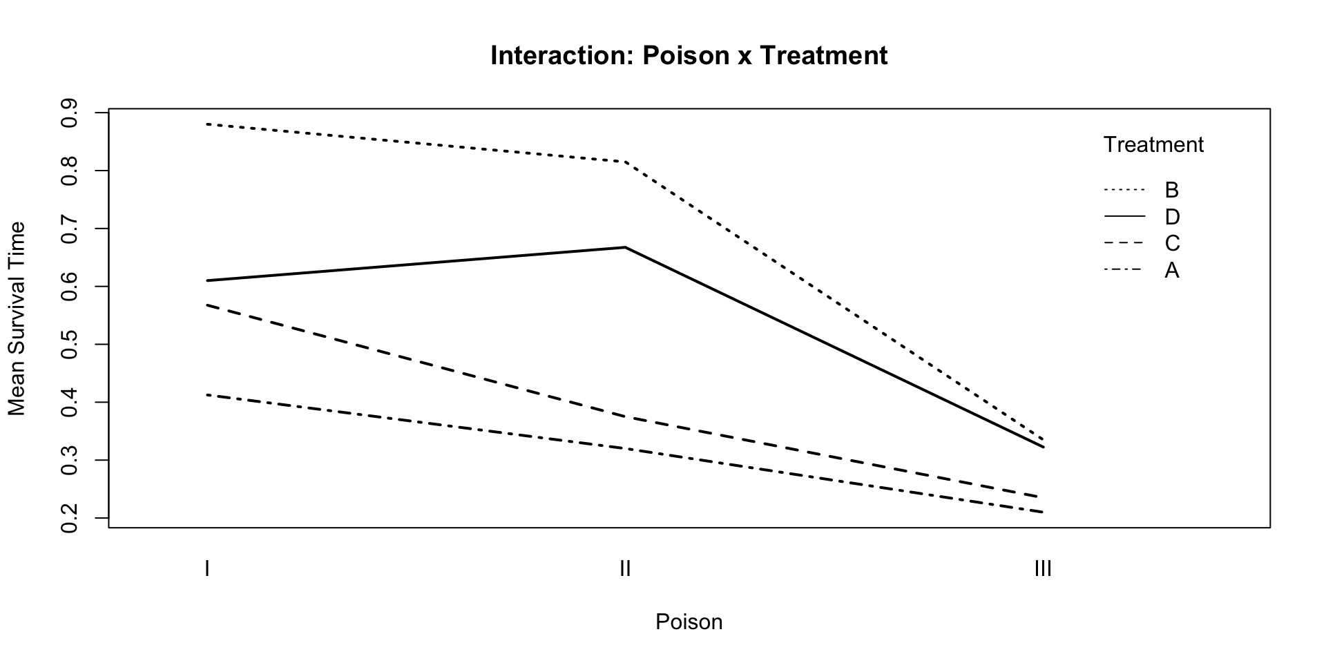
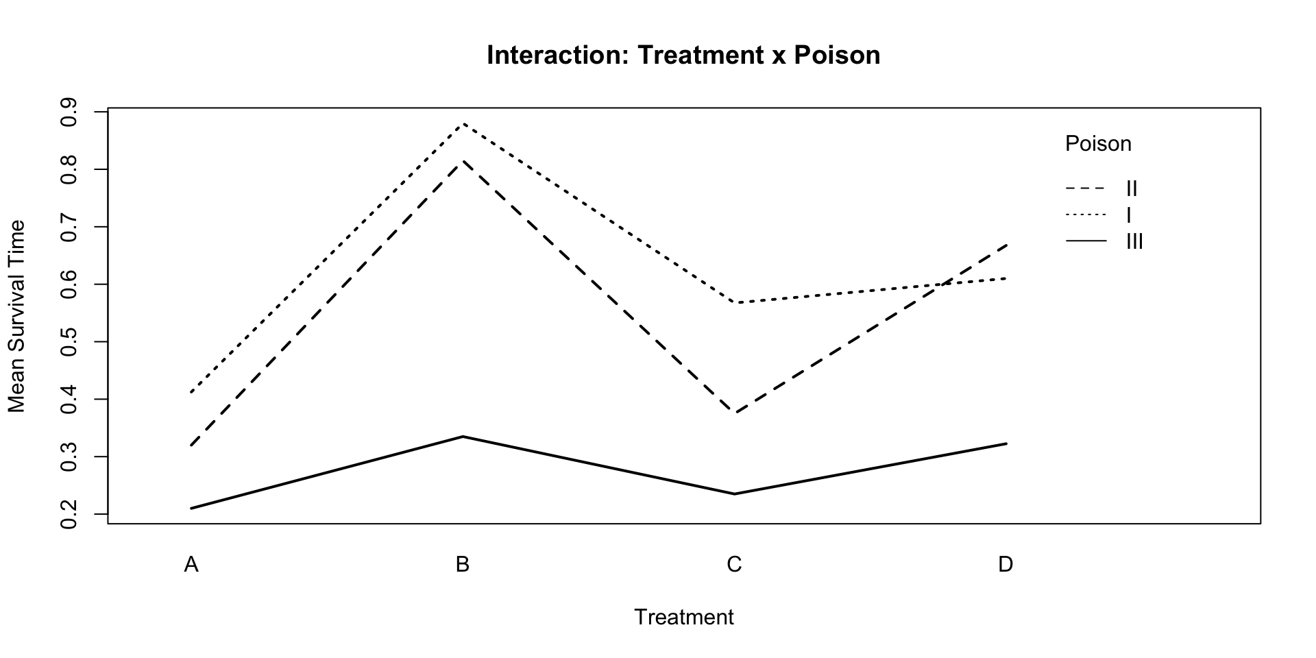
Non-parallel lines suggest interaction.

Two-Way ANOVA with Interaction

L <- aov(Time ~ Poison * Treatment, data=poison)
anova(L)

Analysis of Variance Table

Response: Time
                 Df  Sum Sq Mean Sq F value    Pr(>F)    
Poison            2 1.03708 0.51854 23.3314 3.176e-07 ***
Treatment         3 0.92012 0.30671 13.8000 3.792e-06 ***
Poison:Treatment  6 0.25027 0.04171  1.8768    0.1118    
Residuals        36 0.80010 0.02222                      
---
Signif. codes:  0 '***' 0.001 '**' 0.01 '*' 0.05 '.' 0.1 ' ' 1

Interpretation:

Interaction is not statistically significant (p = 0.1118)
Both main effects are statistically significant

Two-Way ANOVA without Interaction

L1 <- aov(Time ~ Poison + Treatment, data=poison)
anova(L1)

Analysis of Variance Table

Response: Time
          Df  Sum Sq Mean Sq F value    Pr(>F)    
Poison     2 1.03708 0.51854  20.734 5.448e-07 ***
Treatment  3 0.92012 0.30671  12.264 6.743e-06 ***
Residuals 42 1.05037 0.02501                      
---
Signif. codes:  0 '***' 0.001 '**' 0.01 '*' 0.05 '.' 0.1 ' ' 1

# Mean tables
model.tables(L1, type="means")

Tables of means
Grand mean
          
0.4791667 

 Poison 
Poison
     I     II    III 
0.6175 0.5444 0.2756 

 Treatment 
Treatment
     A      B      C      D 
0.3142 0.6767 0.3925 0.5333

Tukey HSD for Two Factors

TukeyHSD(L1, which=c("Poison", "Treatment"))

  Tukey multiple comparisons of means
    95% family-wise confidence level

Fit: aov(formula = Time ~ Poison + Treatment, data = poison)

$Poison
            diff        lwr         upr     p adj
II-I   -0.073125 -0.2089618  0.06271181 0.3987984
III-I  -0.341875 -0.4777118 -0.20603819 0.0000008
III-II -0.268750 -0.4045868 -0.13291319 0.0000582

$Treatment
           diff         lwr        upr     p adj
B-A  0.36250000  0.18980177  0.5351982 0.0000083
C-A  0.07833333 -0.09436490  0.2510316 0.6219967
D-A  0.21916667  0.04646843  0.3918649 0.0079262
C-B -0.28416667 -0.45686490 -0.1114684 0.0004077
D-B -0.14333333 -0.31603157  0.0293649 0.1344032
D-C  0.14083333 -0.03186490  0.3135316 0.1451135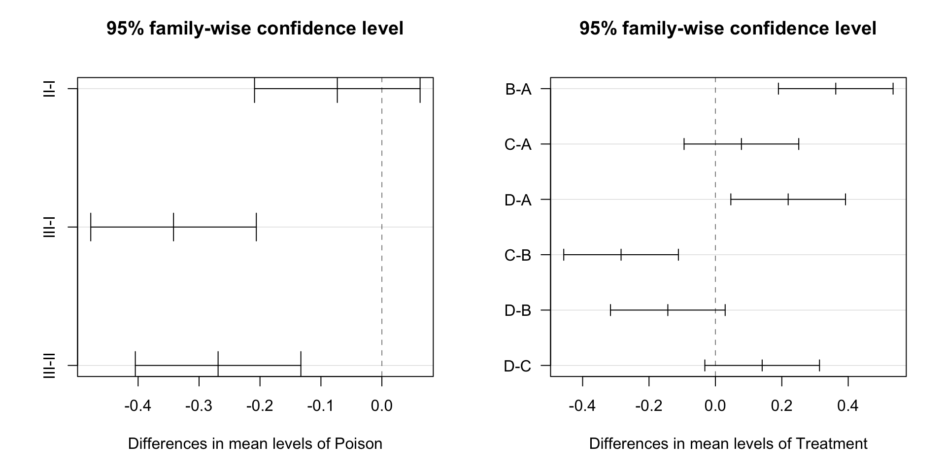

# Visualize
par(mfrow=c(1,2))
plot(TukeyHSD(L1, which="Poison"))
plot(TukeyHSD(L1, which="Treatment"), las=1)

Checking Diagnostics for Two-Way ANOVA

Same assumptions apply! Always check before trusting results.

# Diagnostic plots
par(mfrow=c(2,2))
plot(L1)

# Test assumptions
shapiro.test(residuals(L1))


    Shapiro-Wilk normality test

data:  residuals(L1)
W = 0.92213, p-value = 0.003538

library(car)
leveneTest(Time ~ Poison * Treatment, data=poison)

Levene's Test for Homogeneity of Variance (center = median)
      Df F value    Pr(>F)    
group 11  4.1582 0.0005539 ***
      36                      
---
Signif. codes:  0 '***' 0.001 '**' 0.01 '*' 0.05 '.' 0.1 ' ' 1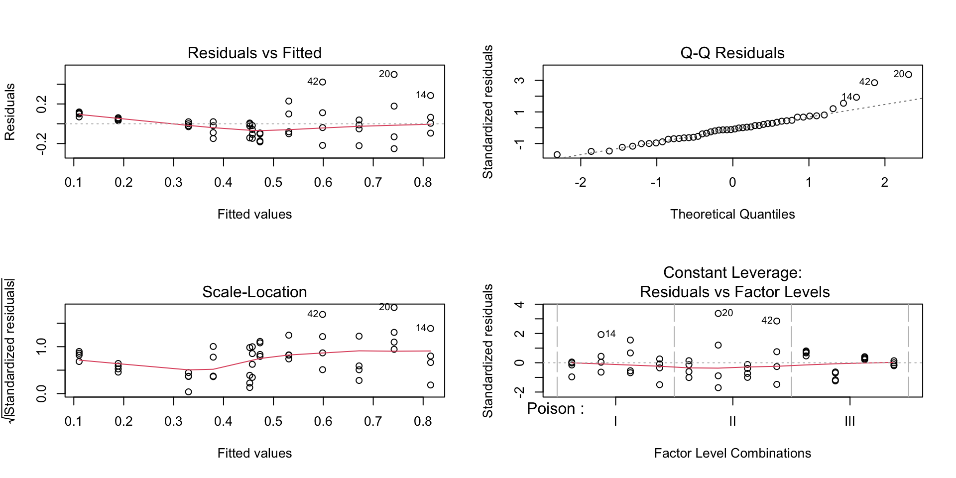

# If assumptions violated, consider transformations
# (as shown earlier in one-way ANOVA)

Note: Two-way ANOVA assumptions are the same as one-way ANOVA!

Part 2 Summary

Key Takeaways:

ANOVA compares means across 3+ groups
Always check assumptions: normality, homogeneity of variance, independence
Use diagnostic plots, Shapiro-Wilk test, and Levene’s test
F-test determines if any differences exist
Multiple comparisons identify which groups differ
Two-way ANOVA examines two factors and their interaction
Transformations or non-parametric tests when assumptions fail

Remember:

Rejecting the null hypothesis in an ANOVA means “not all equal” - use post-hoc tests to find specific differences
Never skip diagnostic checks - violations can invalidate your conclusions!

Final Questions & Next Steps

For next class:

Review model selection and ANOVA concepts
Think about when to use each approach
Practice with your own datasets

Office Hours: After class today

🗓️ Week 05 Model Selection & ANOVA

Part 1: Model Selection & Information Criteria

Class Overview - Part 1

Model Selection: The Problem

Bias-Variance Tradeoff

🎯 Activity 1: Visualizing Overfitting

Model Selection Strategies

Forward Selection

Backward Selection

Stepwise Selection

🎯 Activity 2: Compare Selection Methods

Akaike Information Criterion (AIC)

Bayesian Information Criterion (BIC)

Comparing Models with AIC/BIC

🎯 Activity 3: Build Your Best Model

Cross-Validation: The Gold Standard

Leave-One-Out Cross-Validation (LOOCV)

LOOCV Shortcut for Linear Regression

Cross-Validation in R

🎯 Activity 4: Cross-Validation

Activity 4: Discussion Questions

Alternative: Manual K-Fold CV

Activity 4: Extension Challenge (Optional)

Best Practices for Model Selection

Common Pitfalls to Avoid

❌ Don’t:

✓ Do:

Part 1 Summary

Part 2: Analysis of Variance (ANOVA)

Class Overview - Part 2

One-Way ANOVA

Flicker Data

Exploratory Data Analysis

Visualizing the Data

🎯 Activity 1: Explore the Penguins Data

ANOVA Model: One-Way Design

ANOVA Hypotheses

Partitioning Variance

Sums of Squares

Sums of Squares

F-Statistic and Decision Rule

ANOVA Table

Running ANOVA in R

ANOVA Assumptions

Checking ANOVA Assumptions with Plots

Interpreting ANOVA Diagnostic Plots

Interpreting ANOVA Diagnostic Plots

Testing Normality: Visual and Statistical

Testing Homogeneity of Variance

What to Do When Assumptions Are Violated

What to Do When Assumptions Are Violated

Non-Parametric Alternative: Kruskal-Wallis

Transformations for ANOVA

🎯 Activity 2: Conduct Your Own ANOVA

🎯 Activity 2: Conduct Your Own ANOVA

Multiple Comparisons Problem

Multiple Comparison Methods

Tukey’s HSD in R

Pairwise t-tests with Adjustments

🎯 Activity 3: Multiple Comparisons

Two-Way ANOVA

Poison Data

Interaction Plots

Two-Way ANOVA with Interaction

Two-Way ANOVA without Interaction

Tukey HSD for Two Factors

Checking Diagnostics for Two-Way ANOVA

Part 2 Summary

Final Questions & Next Steps

🗓️ Week 05
Model Selection & ANOVA