🗓️ Week 02
Introduction to R

STAT 204 – Introduction to Statistical Data Analysis

01 Oct 2025

Setting a Seed

For reproducibility:

# Without seed  - different results
rnorm(1)
## [1] 0.4955
rnorm(1)
## [1] -1.3175

# With seed - identical results
set.seed(100)
rnorm(1)
## [1] -0.5022

set.seed(100)
rnorm(1)
## [1] -0.5022

Defining Functions

logit <- function(x){
  z <- log(x/(1-x))
  return(z)
}

logit(runif(3, 0, 1))
## [1]  0.210 -2.818 -0.126

my_norm <- function(x){sqrt(x%*%x)}
my_norm(1:4)
##      [,1]
## [1,] 5.477

Functions with Multiple Arguments

f <- function(x, a=1, b=0){
  a*x^2 + b
}

f(2)        # Uses defaults
## [1] 4

f(2, 2)     # a=2, b=0
## [1] 8

f(2, 2, 2)  # a=2, b=2
## [1] 10

Default values make functions flexible!

Function Internals

To see calculations, use print():

f1 <- function(x){
  paste("Attempt 1 to show value of x=", x)
  print(paste("Attempt 2 to show value of x=", x))
}

f1(3)
## [1] "Attempt 2 to show value of x= 3"

Only printed output is shown!

Function Arguments

Positional vs named:

f <- function(x, y){
  print(paste("x =", x, "y =", y))
}

f(2, 3)
## [1] "x = 2 y = 3"

f(x=2, y=3)
## [1] "x = 2 y = 3"

f(y=3, x=2)
## [1] "x = 2 y = 3"

Lazy Evaluation

R doesn’t check unused arguments:

f <- function(a, b){
  return(a)
}

f(3)        # No error!
## [1] 3

f(3, 2)     # Also works
## [1] 3

Functions as arguments:

summarizex <- function(x, ff){
  z <- ff(x)
  return(z)
}

summarizex(c(1,2,-1,4,0), mean)
## [1] 1.2

Exercise: Functions

Write these functions:

my_range() - takes a vector and returns max - min
standardize() - takes a vector and returns (x - mean)/sd
my_summary() - takes a vector and returns a named list with mean, median, and sd
Post your solution on Ed Discussion

Test your functions on:

test_data <- c(12, 15, 18, 20, 22, 25, 30)

Bonus: Modify my_summary() to handle NA values

Scoping

R allows free variables in functions:

b <- 4
f <- function(x, y){
  z <- x + y/b
  return(z)
}

f(3, 2)
## [1] 3.5

Warning: Avoid free variables unless you know what you’re doing! Can cause unexpected behavior.

Sourcing Functions

Store frequently-used functions in a file:

source(file="myfunctions.R")

Make sure the file is in your working directory or provide full path!

For Loops

for(i in 1:3){
  print(2*i)
}
## [1] 2
## [1] 4
## [1] 6

Index can be any vector:

mystates <- c("CA", "NE", "OR")
for(i in mystates){
  print(i)
}
## [1] "CA"
## [1] "NE"
## [1] "OR"

While Loops

x <- 1
while(x < 10){
  x <- x^2 + 1
  print(x)
}
## [1] 2
## [1] 5
## [1] 26

Efficient Loop Usage

Pre-allocate memory!

# Slow - growing vector
x <- numeric(0)
for(i in 1:10){x[i] = i}

# Even slower - concatenating
x <- numeric(0)
for(i in 1:10){x = c(x,i)}

# Fast - pre-allocated
x <- numeric(10)
for(i in 1:10){x[i] = i}

Memory allocation is expensive!

Loops vs Vectorization

x <- rexp(10000000, rate=1)

logown <- function(x){
  z <- rep(0, length(x))
  for(i in 1:length(x)){
    z[i] <-
       log(x[i])
  }
  return(z)
}

system.time(log(x))
##    user  system elapsed 
##   0.138   0.017   0.155

system.time(logown(x))
##    user  system elapsed 
##   0.609   0.002   0.612

Vectorized functions are much faster!

The `apply` Function

x <- matrix(rnorm(60000), nrow=10000, ncol=6)

apply(x, 2, mean)  # Column means
## [1] -0.0050 -0.0027  0.0141  0.0054 -0.0008  0.0022

Equivalent loop:

z <- numeric(6)
for(i in 1:6){
  z[i] <- mean(x[,i])
}

apply() is cleaner but not always faster!

Apply with Multiple Arguments

x <- matrix(rnorm(6000), ncol=3)

apply(x, 2, quantile, c(0.025, 0.975))
##            [,1]      [,2]      [,3]
## 2.5%  -1.890475 -1.950963 -1.990845
## 97.5%  1.981555  1.977111  1.992657

Additional arguments passed to the function!

Built-in Optimized Functions

For common operations, use optimized functions:

x <- matrix(rexp(6000000), ncol=6000)

system.time(apply(x, 2, sum))
##    user  system elapsed 
##   0.073   0.020   0.092

system.time(colSums(x))
##    user  system elapsed 
##   0.008   0.000   0.008

Much faster!

Exercise: Matrix Standardization

We looked at two different ways to standardize the columns of a matrix:

x <- matrix(rexp(6000000), ncol=6000)

system.time(for(i in 1:6000){x[,i] = x[,i]/sum(x[,i])})
##    user  system elapsed 
##   0.050   0.011   0.061

system.time(scale(x, center=F, scale=colSums(x)))
##    user  system elapsed 
##   0.040   0.005   0.045

Your task: Find a third approach and compare the computation time to the first two approaches. Post your solution on Ed Discussion.

Hint: Consider using sweep() or vectorization with matrix operations

The `expand.grid` Function

Evaluate functions on a 2D grid:

x <- seq(-2, 2, length=50)
y <- seq(-2, 2, length=50)
f <- function(x, y) x^2 + y^2

# This only evaluates diagonal
str(f(x, y))
##  num [1:50] 8 7.36 6.75 6.16 5.6 ...

# This evaluates full grid
z <- expand.grid(x, y)
str(f(z[,1], z[,2]))
##  num [1:2500] 8 7.68 7.37 7.08 6.8 ...

Conditional Statements

x <- 7
if(x <= 10){
  print("Less than or equal to 10!")
} else {
  print("Greater than 10!")
}
## [1] "Less than or equal to 10!"

Logical operators:

if(x <= 10 & x > 5){
  print("Between 5 and 10!")
}
## [1] "Between 5 and 10!"

& = and, | = or

Vectorized Conditionals

x <- c(1, 3, -1)

if(x < 2){print("Hello")} else{print("Bye")}
## Warning: condition has length > 1
## [1] "Hello"

ifelse(x < 2, "Hello", "Bye")
## [1] "Hello" "Bye"   "Hello"

Nested ifelse:

ifelse(x < 2, ifelse(x < 0, "Hello", ""), "Bye")
## [1] ""      "Bye"   "Hello"

Exercise: Function Minimization

Finding the Minimum of a Function

Consider the following function:

$f(x, y) = (1.5 - x + xy)^2 + (2.25 - x + xy^2)^2 + (2.625 - x + xy^3)^2$

where possible inputs for $x$ and $y$ are from -4 to 4 in increments of 0.1.

Your tasks:

Create a grid of all (x, y) combinations using expand.grid()
Evaluate the function at all points in the grid
Find the global minimum - what values of x and y result in this minimum?

Hint: Use which.min() to find the index of the minimum value

Saving Your Work

Save specific objects:

x <- seq(1, 8)
y <- c("CA", "NE")
save(x, y, file="myobjects.R")

Save matrix as text:

x <- matrix(1:10, ncol=5)
write(x, file="myfile.txt")

R packages: Extending R’s power

Working with packages

Packages are collections of functions that extend R:

# Install a package (only need to do this once)
install.packages("tidyverse")

# Load a package (do this each R session)
library(tidyverse)

# Now you can use functions from that package! 🎉

Popular packages 📦

tidyverse: Data manipulation and visualization
ggplot2: Beautiful graphics (part of tidyverse)
dplyr: Data manipulation (part of tidyverse)
palmerpenguins: Practice datasets (including penguins!) 🐧

Getting help in R

Help system

R has excellent built-in help:

# Get help for a function
?mean
help(mean)

# Search for help on a topic
??regression

# See examples of how to use a function
example(mean)

Other ways to get help 🆘

Google: “How to [do something] in R”
Stack Overflow: Huge community of R users
R Documentation: Official function documentation
Your classmates and instructor! 👥
Note about LLMs: Try to avoid them for now. You should learn the basics without using them. Once you feel comfortable using R, it’s up to you. Just please don’t use them now.

Let’s look at real data!

The penguins dataset

# Load the palmerpenguins package
library(palmerpenguins)

# Look at the penguins dataset
penguins

# A tibble: 344 × 8
   species island    bill_length_mm bill_depth_mm flipper_length_mm body_mass_g
   <fct>   <fct>              <dbl>         <dbl>             <int>       <int>
 1 Adelie  Torgersen           39.1          18.7               181        3750
 2 Adelie  Torgersen           39.5          17.4               186        3800
 3 Adelie  Torgersen           40.3          18                 195        3250
 4 Adelie  Torgersen           NA            NA                  NA          NA
 5 Adelie  Torgersen           36.7          19.3               193        3450
 6 Adelie  Torgersen           39.3          20.6               190        3650
 7 Adelie  Torgersen           38.9          17.8               181        3625
 8 Adelie  Torgersen           39.2          19.6               195        4675
 9 Adelie  Torgersen           34.1          18.1               193        3475
10 Adelie  Torgersen           42            20.2               190        4250
# ℹ 334 more rows
# ℹ 2 more variables: sex <fct>, year <int>

# Quick exploration
nrow(penguins)  # How many rows (observations)?

[1] 344

ncol(penguins)  # How many columns (variables)?

[1] 8

names(penguins) # What are the column names?

[1] "species"           "island"            "bill_length_mm"   
[4] "bill_depth_mm"     "flipper_length_mm" "body_mass_g"      
[7] "sex"               "year"

Data exploration functions

# Look at the first few rows
head(penguins)

# A tibble: 6 × 8
  species island    bill_length_mm bill_depth_mm flipper_length_mm body_mass_g
  <fct>   <fct>              <dbl>         <dbl>             <int>       <int>
1 Adelie  Torgersen           39.1          18.7               181        3750
2 Adelie  Torgersen           39.5          17.4               186        3800
3 Adelie  Torgersen           40.3          18                 195        3250
4 Adelie  Torgersen           NA            NA                  NA          NA
5 Adelie  Torgersen           36.7          19.3               193        3450
6 Adelie  Torgersen           39.3          20.6               190        3650
# ℹ 2 more variables: sex <fct>, year <int>

# Get a summary of the data
summary(penguins)

      species          island    bill_length_mm  bill_depth_mm  
 Adelie   :152   Biscoe   :168   Min.   :32.10   Min.   :13.10  
 Chinstrap: 68   Dream    :124   1st Qu.:39.23   1st Qu.:15.60  
 Gentoo   :124   Torgersen: 52   Median :44.45   Median :17.30  
                                 Mean   :43.92   Mean   :17.15  
                                 3rd Qu.:48.50   3rd Qu.:18.70  
                                 Max.   :59.60   Max.   :21.50  
                                 NA's   :2       NA's   :2      
 flipper_length_mm  body_mass_g       sex           year     
 Min.   :172.0     Min.   :2700   female:165   Min.   :2007  
 1st Qu.:190.0     1st Qu.:3550   male  :168   1st Qu.:2007  
 Median :197.0     Median :4050   NA's  : 11   Median :2008  
 Mean   :200.9     Mean   :4202                Mean   :2008  
 3rd Qu.:213.0     3rd Qu.:4750                3rd Qu.:2009  
 Max.   :231.0     Max.   :6300                Max.   :2009  
 NA's   :2         NA's   :2

# Look at the structure of the data
str(penguins)

tibble [344 × 8] (S3: tbl_df/tbl/data.frame)
 $ species          : Factor w/ 3 levels "Adelie","Chinstrap",..: 1 1 1 1 1 1 1 1 1 1 ...
 $ island           : Factor w/ 3 levels "Biscoe","Dream",..: 3 3 3 3 3 3 3 3 3 3 ...
 $ bill_length_mm   : num [1:344] 39.1 39.5 40.3 NA 36.7 39.3 38.9 39.2 34.1 42 ...
 $ bill_depth_mm    : num [1:344] 18.7 17.4 18 NA 19.3 20.6 17.8 19.6 18.1 20.2 ...
 $ flipper_length_mm: int [1:344] 181 186 195 NA 193 190 181 195 193 190 ...
 $ body_mass_g      : int [1:344] 3750 3800 3250 NA 3450 3650 3625 4675 3475 4250 ...
 $ sex              : Factor w/ 2 levels "female","male": 2 1 1 NA 1 2 1 2 NA NA ...
 $ year             : int [1:344] 2007 2007 2007 2007 2007 2007 2007 2007 2007 2007 ...

Interactive data exploration

Explore the penguins! (8 minutes) 🐧

Working with a partner:

Use View(penguins) to open the data in a spreadsheet-like view
How many penguin species are in the data?
What’s the average bill length? (Hint: mean(penguins$bill_length_mm, na.rm = TRUE))
What islands are represented?
How many penguins are from each island? (Hint: table(penguins$island))

Discuss: What interesting patterns do you notice? 🔍

Importing Data: Manual Entry

For small datasets:

y1 <- c(22, 26)
y2 <- c(28, 24, 29)
y3 <- c(29, 32, 28)
y4 <- c(23, 24)

y <- c(y1, y2, y3, y4)
Model <- c(rep("A", 2), rep("B", 3), rep("C", 3), rep("D", 2))
mileages <- data.frame(y, Model)

Importing from Files

Text file with headers:

arod <- read.table("data/a-rod-2016.txt", header=T)

CSV files:

data <- read.csv("mydata.csv")

Tips for preparing data:

Same number of columns per row
Use NA for missing data
Remove special characters
Replace spaces in headers with underscores

Reformatting Data

df <- PlantGrowth
unstacked_df <- unstack(df)
head(unstacked_df, 3)
##   ctrl trt1 trt2
## 1 4.17 4.81 6.31
## 2 5.58 4.17 5.12
## 3 5.18 4.41 5.54

stacked_df <- stack(unstacked_df)
head(stacked_df, 3)
##   values  ind
## 1   4.17 ctrl
## 2   5.58 ctrl
## 3   5.18 ctrl

Merging Data Frames

authors <- data.frame(
  surname = c("Tukey", "Venables", "Tierney", "Ripley", "McNeil"), 
  nationality = c("US", "AUS", "US", "UK", "AUS")
)

books <- data.frame(
  name = c("Tukey", "Venables", "Tierney", "Ripley", "Ripley", "McNeil", "R Core"), 
  title = c("Exploratory Data Analysis", "Modern Applied Statistics", 
            "LISP-STAT", "Spatial Statistics", "Stochastic Simulation", 
            "Interactive Data Analysis", "An Introduction to R")
)

m1 <- merge(authors, books, by.x = "surname", by.y = "name")

Merge Result

m1
##    surname nationality                         title
## 1   McNeil         AUS   Interactive Data Analysis
## 2   Ripley          UK          Spatial Statistics
## 3   Ripley          UK         Stochastic Simulation
## 4  Tierney          US                     LISP-STAT
## 5    Tukey          US     Exploratory Data Analysis
## 6 Venables         AUS Modern Applied Statistics

Only matching rows are kept by default!

Numerical Summaries

Data Types

A variable may be classified as:

Quantitative: numeric or integer
Ordinal: an ordered categorical variable (e.g., low/medium/high)
Qualitative: categorical, nominal, or factors

A dataframe may contain variables of different types.

Data may have additional structure as well. For example, when data are collected over time, we have time series data which is indexed by time. Similarly, when data are collected over a spatial domain, we have spatial data which is indexed by a location.

Data Summary

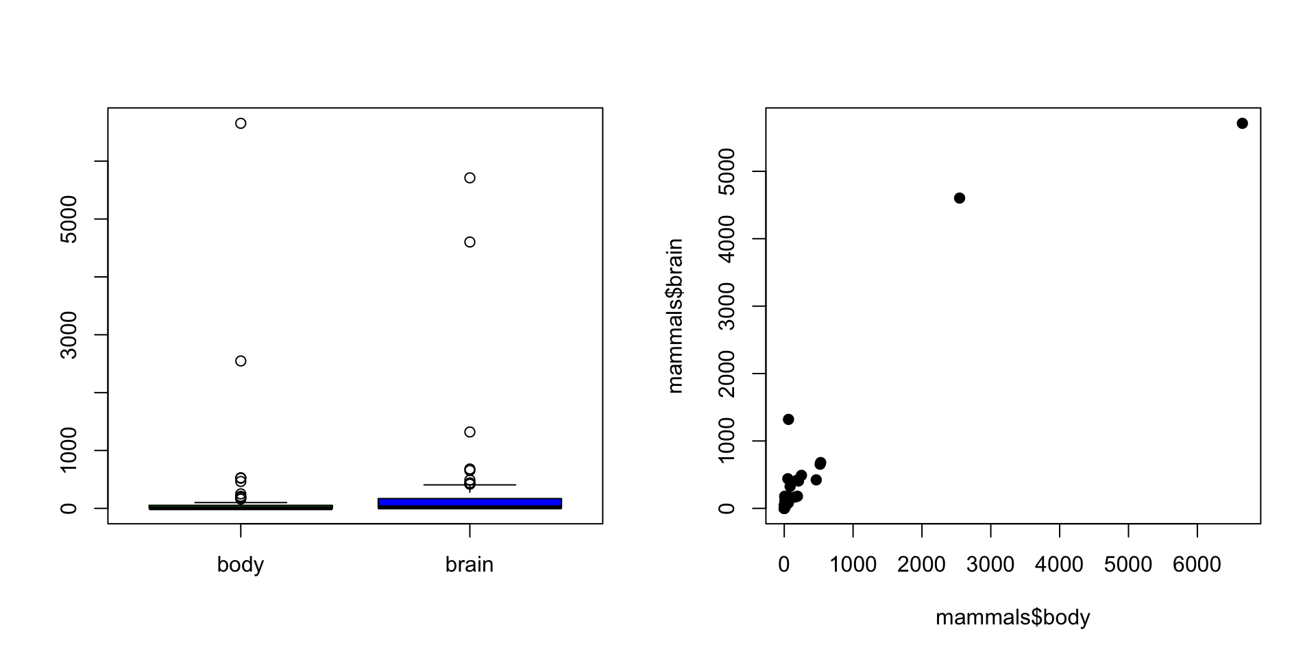
Example: body and brain size of mammals (two quantitative variables)

library(MASS)
head(mammals) # you can use ?mammals to get more info

                   body brain
Arctic fox        3.385  44.5
Owl monkey        0.480  15.5
Mountain beaver   1.350   8.1
Cow             465.000 423.0
Grey wolf        36.330 119.5
Goat             27.660 115.0

summary(mammals) # very skewed data

      body              brain        
 Min.   :   0.005   Min.   :   0.14  
 1st Qu.:   0.600   1st Qu.:   4.25  
 Median :   3.342   Median :  17.25  
 Mean   : 198.790   Mean   : 283.13  
 3rd Qu.:  48.203   3rd Qu.: 166.00  
 Max.   :6654.000   Max.   :5712.00

Basic Graphical Summaries

par(mfrow=c(1,2))
boxplot(mammals, col=c('green', 'blue'))
plot(mammals$body,mammals$brain, pch=19)

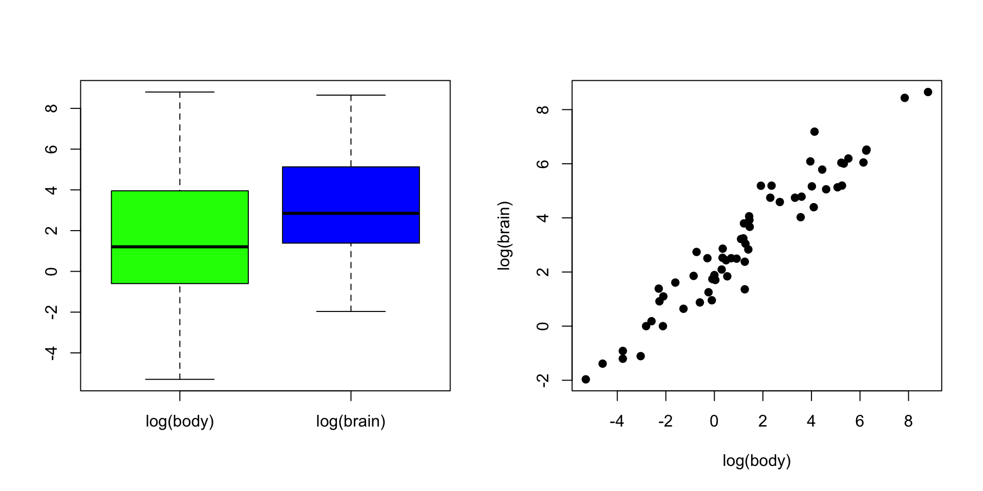
Basic Graphical Summaries

par(mfrow=c(1,2))
boxplot(log(mammals), names=c("log(body)", "log(brain)"),
        col=c('green', 'blue'))
plot(log(mammals$body),log(mammals$brain), pch=19,
     ylab="log(brain)", xlab="log(body)")

Correlation

\[\rho_{X,Y} = \frac{\text{Cov}(X, Y)}{\text{SD}(X) \times \text{SD}(Y)} = \frac{E[(X - \mu_X)(Y - \mu_Y)]}{\sigma_X \sigma_Y}\]

\[r_{xy} = \frac{S_{xy}}{\sqrt{S_{xx}S_{yy}}}\]

where:

$S_{xx} = \sum_{i=1}^{n}(x_i - \bar{x})^2$, $\bar{x} = \frac{\sum_{i=1}^{n} x_i}{n}$
$S_{xy} = \sum_{i=1}^{n}(x_i - \bar{x})(y_i - \bar{y})$
$S_{yy} = \sum_{i=1}^{n}(y_i - \bar{y})^2$, $\bar{y} = \frac{\sum_{i=1}^{n} y_i}{n}$

Correlation Example

cor(mammals)

           body     brain
body  1.0000000 0.9341638
brain 0.9341638 1.0000000

cor(log(mammals))

           body     brain
body  1.0000000 0.9595748
brain 0.9595748 1.0000000

Bivariate Data by Group

Example: IQ of twins separated near birth

library(UsingR)
# Foster: IQ for twin raised with foster parents
# Biological: IQ for twin raised with biological parents
# Social: Social status of biological parent
twins

   Foster Biological Social
1      82         82   high
2      80         90   high
3      88         91   high
4     108        115   high
5     116        115   high
6     117        129   high
7     132        131   high
8      71         78 middle
9      75         79 middle
10     93         82 middle
11     95         97 middle
12     88        100 middle
13    111        107 middle
14     63         68    low
15     77         73    low
16     86         81    low
17     83         85    low
18     93         87    low
19     97         87    low
20     87         93    low
21     94         94    low
22     96         95    low
23    112         97    low
24    113         97    low
25    106        103    low
26    107        106    low
27     98        111    low

Example

Numeric Summary

summary(twins)

     Foster         Biological       Social  
 Min.   : 63.00   Min.   : 68.0   high  : 7  
 1st Qu.: 84.50   1st Qu.: 83.5   low   :14  
 Median : 94.00   Median : 94.0   middle: 6  
 Mean   : 95.11   Mean   : 95.3              
 3rd Qu.:107.50   3rd Qu.:104.5              
 Max.   :132.00   Max.   :131.0

Boxplots of the difference in IQ by social status

boxplot(Foster - Biological ~ Social, twins)

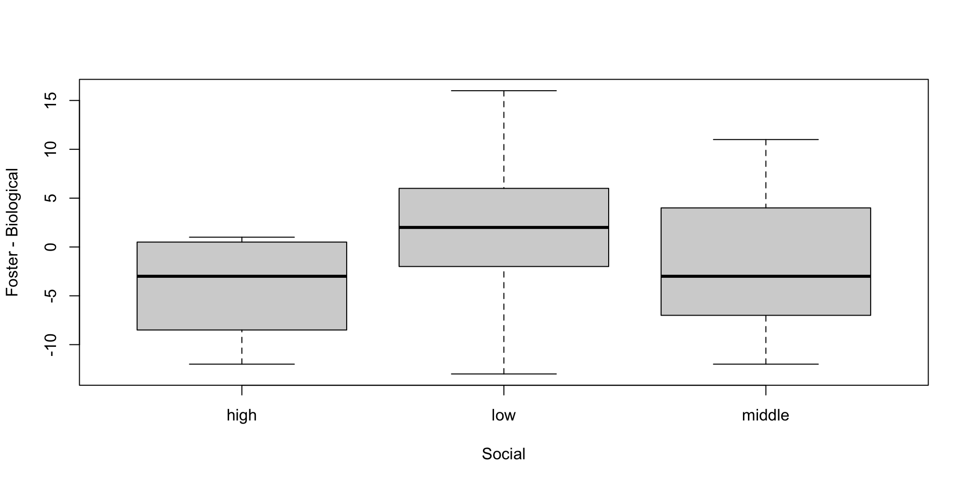
Example Continued

Another way to display this data is through a scatterplot

attach(twins)
plot(x=Foster, y=Biological, pch=as.integer(Social),
     col=as.integer(Social))
legend("topleft", c("high", "low", "middle"), pch=1:3,
       col=1:3, inset=.02)
abline(0,1)

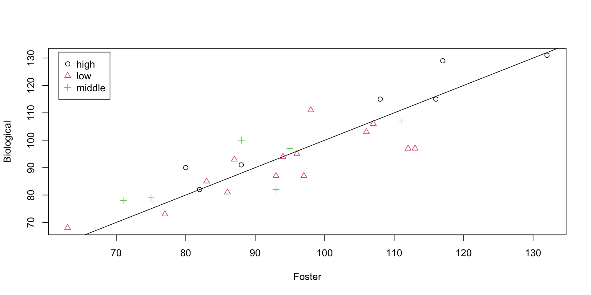
Conditional Plots

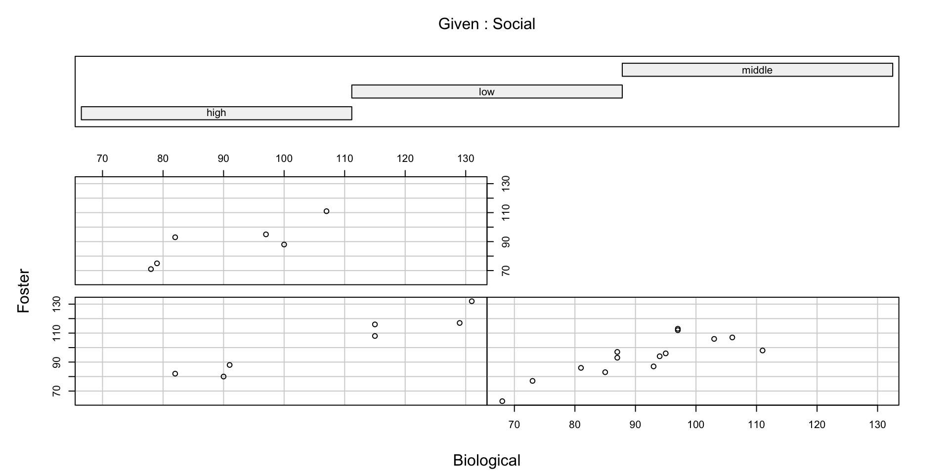
The function coplot displays several plots on the same scale. The syntax y~x|a means plots of y vs. x are conditional on a (order from bottom and from left)

coplot(Foster ~ Biological|Social, data=twins)

Conditional Plots

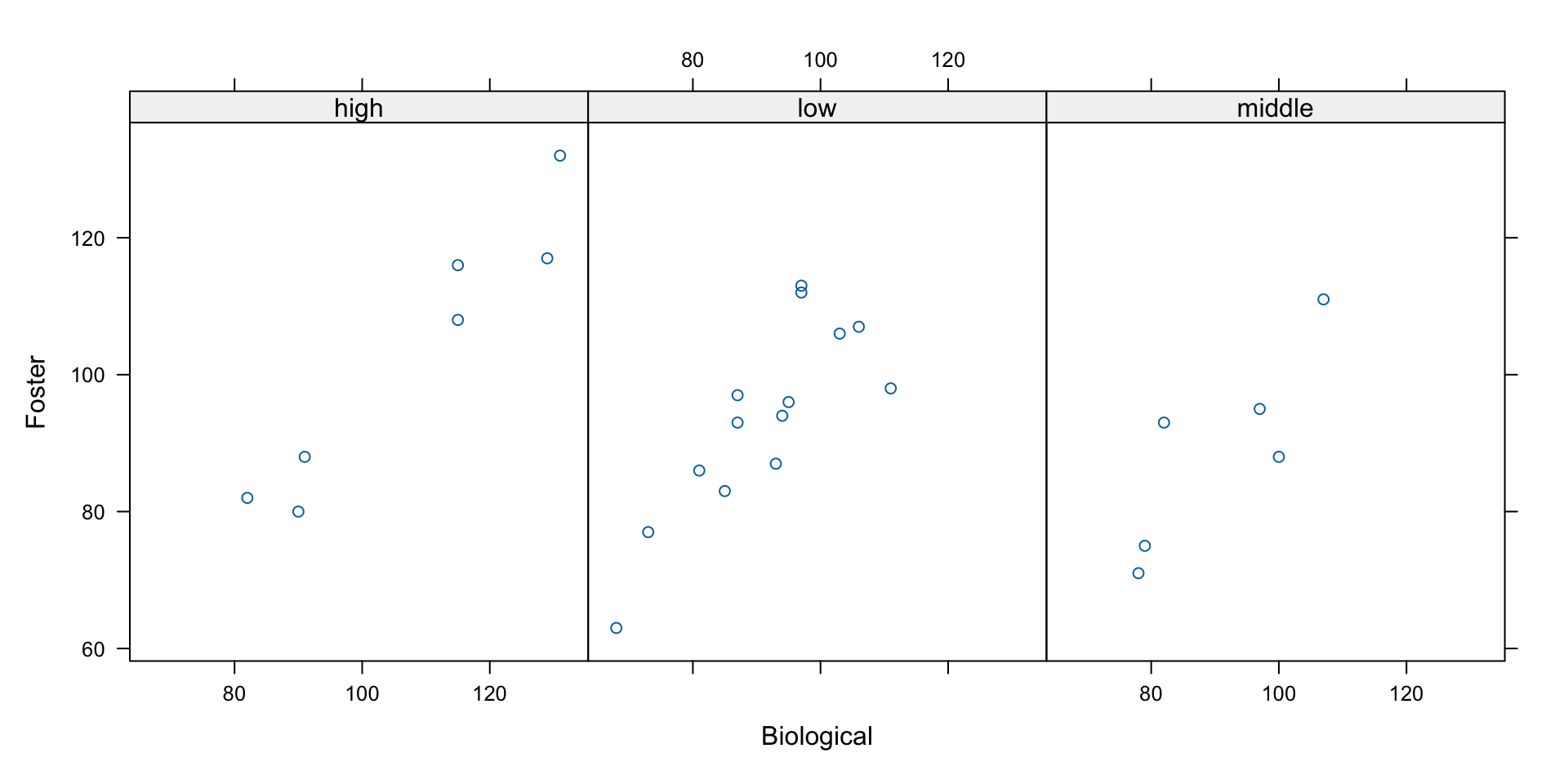
the lattice library also allows us to make conditional plots, which may be easier to read

library(lattice)
xyplot(Foster ~ Biological|Social, data=twins)

Activity 1: Exploring the Twins Dataset

Working with your neighbor (8 minutes)

Let’s explore the twins dataset from the UsingR package:

library(UsingR)
data(twins)

Your tasks:

Calculate the mean and standard deviation for Foster and Biological IQ scores
Create side-by-side boxplots comparing Foster vs Biological IQs
Calculate the difference: IQ_diff <- twins$Foster - twins$Biological
What percentage of twins raised by foster parents have higher IQs than their biological twin?

Post your findings on Ed Discussion!

Multivariate Data

Example: data from a study comparing brain size and intelligence; 40 individuals; brain size measured by MRI; 8 variables

Here’s the table in proper markdown format:

Variable	Description
Gender	Male or Female
FSIQ	Full Scale IQ scores based on four Wechsler (1981) subtests
VIQ	Verbal IQ scores based on four Wechsler (1981) subtests
PIQ	Performance IQ scores based on four Wechsler (1981) subtests
Weight	Body weight in pounds
Height	Height in inches
MRI_Count	total pixel Count from the 18 MRI scans

Example

Note the missing values under weight and height

brain <- read.csv('data/brain.csv')
summary(brain)

    Gender               FSIQ             VIQ             PIQ        
 Length:40          Min.   : 77.00   Min.   : 71.0   Min.   : 72.00  
 Class :character   1st Qu.: 89.75   1st Qu.: 90.0   1st Qu.: 88.25  
 Mode  :character   Median :116.50   Median :113.0   Median :115.00  
                    Mean   :113.45   Mean   :112.3   Mean   :111.03  
                    3rd Qu.:135.50   3rd Qu.:129.8   3rd Qu.:128.00  
                    Max.   :144.00   Max.   :150.0   Max.   :150.00  
                                                                     
     Weight          Height        MRI_Count      
 Min.   :106.0   Min.   :62.00   Min.   : 790619  
 1st Qu.:135.2   1st Qu.:66.00   1st Qu.: 855918  
 Median :146.5   Median :68.00   Median : 905399  
 Mean   :151.1   Mean   :68.53   Mean   : 908755  
 3rd Qu.:172.0   3rd Qu.:70.50   3rd Qu.: 950078  
 Max.   :192.0   Max.   :77.00   Max.   :1079549  
 NA's   :2       NA's   :1

Example Continued

Missing values:

The by function allows us to consider summaries by group

mean(brain$Weight)

[1] NA

mean(brain$Weight, na.rm=T)

[1] 151.0526

by(data=brain$PIQ, INDICES = brain$Gender, FUN=mean, na.rm=T)

brain$Gender: Female
[1] 110.45
------------------------------------------------------------ 
brain$Gender: Male
[1] 111.6

Example Continued

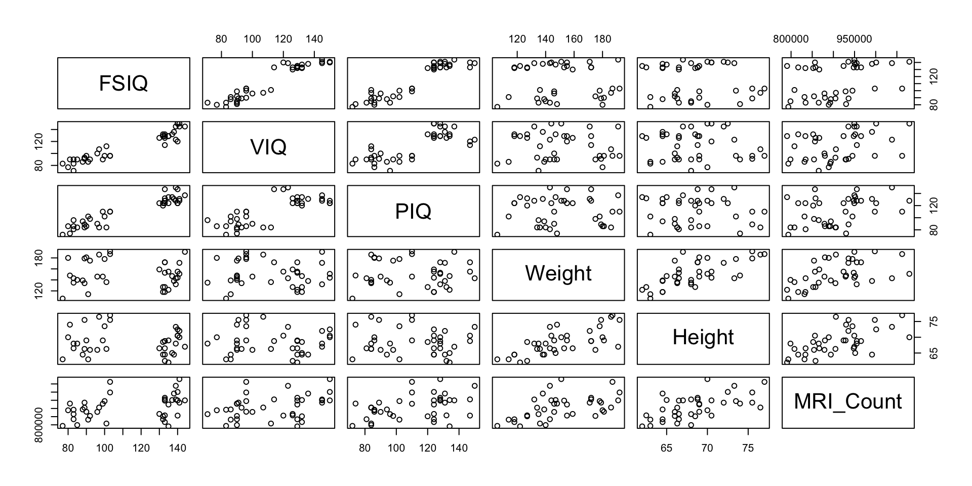
The pairs function can be used to display scatterplots for all pairs of (numeric) variables

pairs(brain[,-1])

Example Continued

The variables FSIQ, VIQ, and PIQ have strong positive correlation

round(cor(brain[,-1]), 2)

          FSIQ  VIQ  PIQ Weight Height MRI_Count
FSIQ      1.00 0.95 0.93     NA     NA      0.36
VIQ       0.95 1.00 0.78     NA     NA      0.34
PIQ       0.93 0.78 1.00     NA     NA      0.39
Weight      NA   NA   NA      1     NA        NA
Height      NA   NA   NA     NA      1        NA
MRI_Count 0.36 0.34 0.39     NA     NA      1.00

round(cor(brain[,-1], use="pairwise.complete.obs"), 2)

           FSIQ   VIQ   PIQ Weight Height MRI_Count
FSIQ       1.00  0.95  0.93  -0.05  -0.09      0.36
VIQ        0.95  1.00  0.78  -0.08  -0.07      0.34
PIQ        0.93  0.78  1.00   0.00  -0.08      0.39
Weight    -0.05 -0.08  0.00   1.00   0.70      0.51
Height    -0.09 -0.07 -0.08   0.70   1.00      0.60
MRI_Count  0.36  0.34  0.39   0.51   0.60      1.00

Example Continued

Controlling for body size (measured as weight): Identifying missing data:

attach(brain)
mri <- MRI_Count/Weight
cor(FSIQ, mri, use="pairwise.complete.obs")

[1] 0.235308

which(is.na(brain), arr.ind=T)

     row col
[1,]   2   5
[2,]  21   5
[3,]  21   6

brain[21,]

   Gender FSIQ VIQ PIQ Weight Height MRI_Count
21   Male   83  83  86     NA     NA    892420

Activity 2: Brain Size and Intelligence

Partner work (10 minutes)

Investigate the relationship between brain size and IQ scores:

brain <- read.csv('data/brain.csv')

Your tasks:

Create a scatterplot of MRI_Count (x-axis) vs FSIQ (y-axis)
Calculate the correlation between MRI_Count and FSIQ (remember to handle missing values!)
Color points by Gender: plot(..., col=as.integer(as.factor(Gender)))
Add a legend to distinguish Male vs Female
Calculate the correlation separately for males and females using by()

Bonus: Control for body size by creating MRI_per_Weight <- MRI_Count/Weight and recalculate the correlation with FSIQ. Does this change your conclusions?

Share your insights on Ed Discussion!

Questions?

Resources:

R Documentation: ?function_name
Help search: ??keyword
Stack Overflow for R
R for Data Science book

Practice makes perfect!

🗓️ Week 02 Introduction to R

Setting a Seed

Defining Functions

Functions with Multiple Arguments

Function Internals

Function Arguments

Lazy Evaluation

Exercise: Functions

Scoping

Sourcing Functions

For Loops

While Loops

Efficient Loop Usage

Loops vs Vectorization

The apply Function

Apply with Multiple Arguments

Built-in Optimized Functions

Exercise: Matrix Standardization

The expand.grid Function

Conditional Statements

Vectorized Conditionals

Exercise: Function Minimization

Saving Your Work

R packages: Extending R’s power

Working with packages

Getting help in R

Help system

Let’s look at real data!

The penguins dataset

Data exploration functions

Interactive data exploration

Importing Data: Manual Entry

Importing from Files

Reformatting Data

Merging Data Frames

Merge Result

Numerical Summaries

Data Types

Data Summary

Basic Graphical Summaries

Basic Graphical Summaries

Correlation

Correlation Example

Bivariate Data by Group

Example

Example Continued

Conditional Plots

Conditional Plots

Activity 1: Exploring the Twins Dataset

Multivariate Data

Example

Example Continued

Example Continued

Example Continued

Example Continued

Activity 2: Brain Size and Intelligence

Questions?

🗓️ Week 02
Introduction to R

The `apply` Function

The `expand.grid` Function