STAT 17: Statistical Methods for Business and Economics
08 Jun 2026
📊 Case Study: TechStart Ventures (Continued)
The Next Challenge
Last time, we found:
Strong correlation (r = 0.85) between advertising and revenue
Regression equation: \(\widehat{\text{Revenue}} = 12.45 + 0.78 \times \text{Advertising}\)
But the investors ask:
- Is this relationship statistically significant? Or could it be due to chance?
- How confident can we be in our predictions?
- Could the true slope actually be zero in the population?
- What’s the margin of error for our revenue forecasts?
Today: Move from description to inference - test hypotheses and quantify uncertainty!
Learning Objectives 🎯
By the end of today’s lecture, you will be able to:
- Understand the assumptions/conditions for regression inference
- Test hypotheses about the population slope (\(\beta_1\))
- Interpret p-values and t-statistics in regression
- Calculate and interpret confidence intervals for slope
- Understand standard error of regression
- Assess statistical significance of relationships
- Understand multiple linear regression basics
Review: What We Know So Far
Sample Statistics (Descriptive)
- Sample correlation: \(r = 0.85\)
- Sample slope: \(b_1 = 0.78\)
- Sample intercept: \(b_0 = 12.45\)
- Sample R²: \(R^2 = 0.72\)
These describe our sample data
Population Parameters (Inferential)
- Population correlation: \(\rho\) (rho)
- Population slope: \(\beta_1\) (beta)
- Population intercept: \(\beta_0\) (beta)
- Population R²: not typically estimated
These are the true values we want to know
Important
Key Question: Can we use our sample statistics to make inferences about population parameters?
The Sampling Distribution of \(b_1\)
If we took many different samples and calculated \(b_1\) each time:
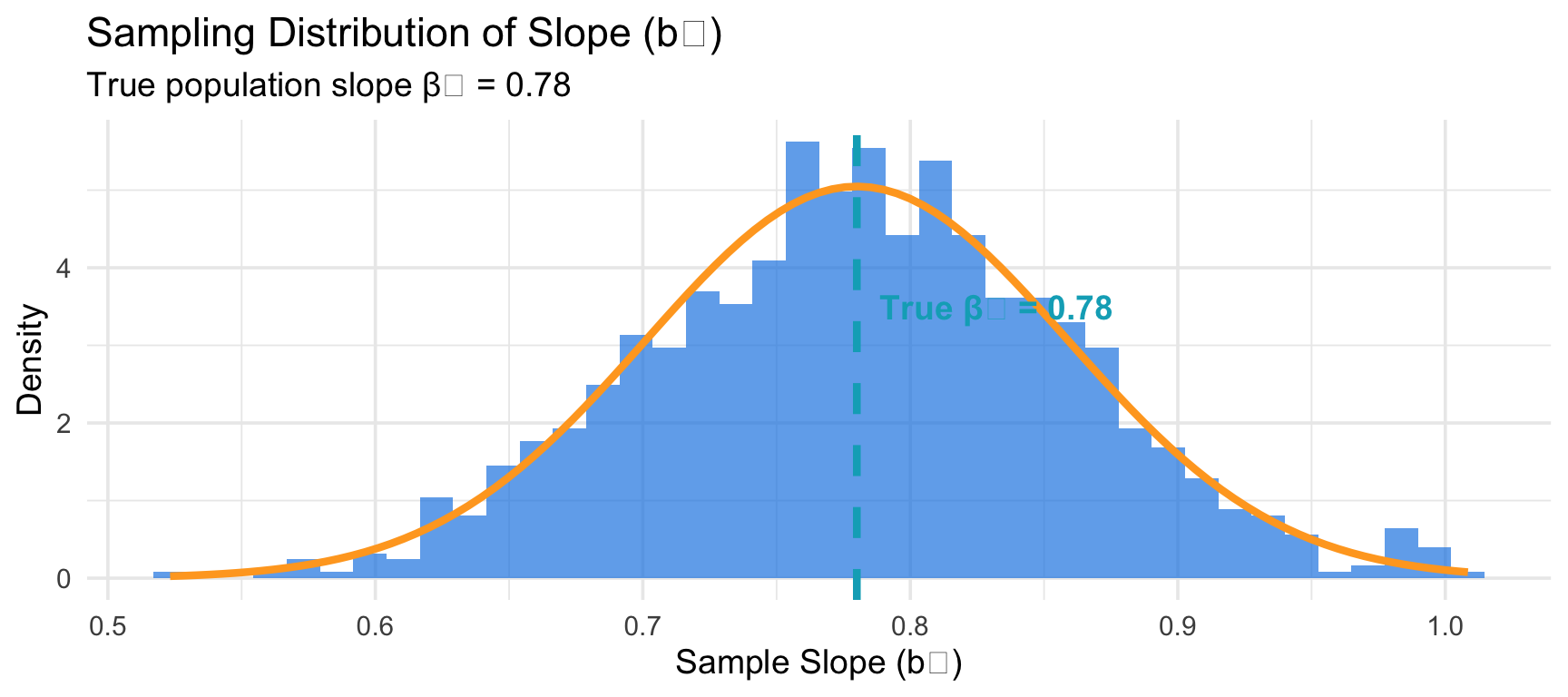
Key insight: \(b_1\) varies from sample to sample, but centers around the true \(\beta_1\)!
Conditions for Regression Inference
Before doing inference, check these conditions:
- Linearity: Relationship between x and y is linear
- Check: Scatterplot shows linear pattern
- Independence: Observations are independent
- Check: Random sampling, no time series
- Normality: Residuals are approximately normally distributed
- Check: Histogram or normal probability plot of residuals
- Less important with large samples (n > 30)
- Equal variance (Homoscedasticity): Spread of residuals is constant
- Check: Residual plot shows no fan/cone shape
Warning
Mnemonic: LINE (Linearity, Independence, Normality, Equal variance)
Checking Conditions: Residual Plot
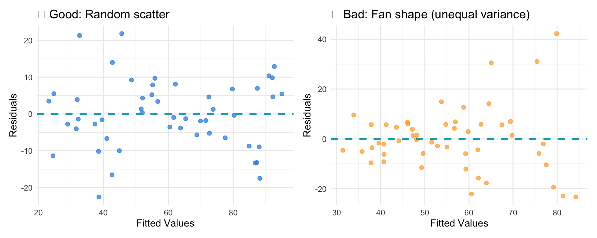
What to look for:
- Good: Random scatter around zero, no patterns
- Bad: Fan/cone shape, curves, clusters
THINK-PAIR-SHARE 1 (5 minutes)
Which condition is MOST important to check before regression inference?
A. The residuals are perfectly normal
B. The relationship is linear
C. Every single data point is independent
D. R² is above 0.70

Part 1: Testing Hypotheses About Slope
Is the relationship statistically significant?
Hypothesis Test for Slope (\(\beta_1\))
Standard Test Setup
Hypotheses: \[H_0: \beta_1 = 0\] (No linear relationship in population) \[H_a: \beta_1 \neq 0\] (Linear relationship exists)
Test Statistic: \[t = \frac{b_1 - 0}{SE_{b_1}}\]
where \(SE_{b_1}\) is the standard error of the slope
Degrees of freedom: \(df = n - 2\)
For TechStart: With n = 25 startups, df = 23
Understanding Standard Error of Slope
Standard Error (\(SE_{b_1}\)): Measures variability of slope estimates across samples
\[SE_{b_1} = \frac{s_e}{s_x \sqrt{n-1}}\]
where:
- \(s_e\) = standard error of the regression (residual standard error)
- \(s_x\) = standard deviation of x
- \(n\) = sample size
What affects \(SE_{b_1}\)?
Decreases when: - Residuals are smaller (\(s_e\) ↓) - X has more spread (\(s_x\) ↑) - Sample size is larger (\(n\) ↑)
Result: More precise slope estimate!
TechStart Example: Testing Significance
Given regression output from Google Sheets:
- Sample slope: \(b_1 = 0.78\)
- Standard error: \(SE_{b_1} = 0.12\)
- n = 25 startups
Calculate t-statistic:
\[t = \frac{b_1 - 0}{SE_{b_1}} = \frac{0.78 - 0}{0.12} = 6.50\]
Find p-value: With df = 23, using software: p-value < 0.001
Decision: Reject \(H_0\) at α = 0.05
Conclusion: There is strong evidence of a significant positive linear relationship between advertising and revenue in the population (t = 6.50, p < 0.001).
Interpreting P-values in Regression
P-value: Probability of getting a slope as extreme as ours (or more) if true slope is zero
Small p-value (< \(\alpha\))
- Statistical evidence against \(H_0\)
- Relationship is statistically significant
- Slope is likely NOT zero
- Can use model for prediction
TechStart: p < 0.001
→ Statistical evidence!
Large p-value (≥ \(\alpha\))
- Weak evidence against \(H_0\)
- Relationship is not statistically significant
- Can’t rule out zero slope
- Be cautious about predictions
Example: p = 0.23
→ Not significant
Warning
Statistical significance ≠ Practical significance!
THINK-PAIR-SHARE 2 (5 minutes)
Regression output shows: \(b_1 = 0.45\), \(SE_{b_1} = 0.30\), p-value = 0.15
What should we conclude at α = 0.05?
A. The relationship is statistically significant
B. The relationship is not statistically significant
C. We need more data to decide
D. The slope is definitely zero
Part 2: Confidence Intervals for Slope
Quantifying Uncertainty
Confidence Interval for \(\beta_1\)
Formula
\[b_1 \pm t^* \times SE_{b_1}\]
where:
- \(b_1\) = sample slope
- \(t^*\) = critical value from t-distribution with df = n - 2
- \(SE_{b_1}\) = standard error of slope
For TechStart (95% CI with df = 23):
- \(b_1 = 0.78\), \(SE_{b_1} = 0.12\)
- \(t^* = 2.069\) (from software)
\[0.78 \pm 2.069(0.12) = 0.78 \pm 0.25 = (0.53, 1.03)\]
Interpretation: We are 95% confident that for each additional $1,000 in advertising, revenue increases between $530 and $1,030 in the population.
Confidence Intervals and Hypothesis Tests
Important Connection
For a two-tailed test at significance level α:
If the \((1-\alpha) \times 100\%\) confidence interval for \(\beta_1\):
- Does NOT contain 0 → Reject \(H_0\) (statistically significant relationship)
- Contains 0 → Fail to reject \(H_0\) (not significant)
TechStart example:
- 95% CI: (0.53, 1.03)
- Does NOT contain 0
- Therefore: Reject \(H_0\) at α = 0.05 ✓
This provides more information than hypothesis test alone!
Part 3: Standard Error and Prediction Intervals
Quantifying Prediction Uncertainty
Standard Error of the Regression (\(s_e\))
Measures typical size of prediction errors (residuals)
\[s_e = \sqrt{\frac{\sum(y_i - \widehat{y}_i)^2}{n-2}} = \sqrt{\frac{\text{Sum of Squared Residuals}}{df}}\]
For TechStart
\(s_e = 9.8\) thousand dollars
Interpretation: Estimations are typically off by about $9,800, either direction
Two Types of Intervals
Confidence Interval for Mean Response
Question: What’s the average y for a given \(x_i\)?
Example: What’s the average revenue for ALL startups spending $50k on ads?
Formula: \[\widehat{y} \pm t^* \times s_e \left(\sqrt{ \frac{1}{n}+\frac{(x_i - \bar{x})^2}{s_x}}\right)\]
Narrower interval
(more precise)
Prediction Interval for Individual Response
Question: What y will we observe for a new case?
Example: What revenue will THIS specific startup with $50k ad spending achieve?
Formula: \[\widehat{y} \pm t^* \times s_e \left(\sqrt{ 1+ \frac{1}{n}+\frac{(x_i - \bar{x})^2}{s_x}}\right)\]
Wider interval
(more uncertainty)
Prediction Interval Example
Predict revenue for a startup spending $50,000 on advertising:
Point estimate: \[\widehat{\text{Revenue}} = 12.45 + 0.78(50) = 51.45 \text{ thousand}\]
95% Prediction Interval: (30.8, 72.1) thousand
Interpretation: We are 95% confident this specific startup will generate between $30,800 and $72,100 in revenue.
Note: Wide interval reflects uncertainty in predicting individual cases!
Warning
Key Business Insight: Even with strong correlation (r = 0.85), individual predictions have substantial uncertainty. Don’t over-rely on point estimates!
THINK-PAIR-SHARE 3 (5 minutes)
Why is a prediction interval wider than a confidence interval at the same x value?
A. Because we use a larger t* value
B. Because it accounts for both estimation uncertainty AND individual variation
C. Because the sample size is smaller
D. Because predictions are less accurate
Reading Regression Output
Example output for TechStart:
| Coefficient | Estimate | Std Error | t-stat | p-value |
|---|---|---|---|---|
| Intercept | 12.45 | 3.82 | 3.26 | 0.004 |
| Advertising | 0.78 | 0.12 | 6.50 | < 0.001 |
Additional statistics:
- R² = 0.72
- \(s_e\) = 9.8
- df = 23
What this tells us:
- Both intercept and slope are statistically significant (p < 0.05)
- Advertising coefficient: \(b_1 = 0.78 \pm 2.069(0.12)\) → 95% CI: (0.53, 1.03)
- Model explains 72% of variance
- Typical prediction error: $9,800
Complete Inference Example
TechStart Ventures: Full Analysis
Research Question: Is advertising spending significantly related to revenue?
1. Check Conditions: - ✓ Linearity: Scatterplot shows linear pattern - ✓ Independence: Random sample of startups - ✓ Normality: Residuals approximately normal (n = 25) - ✓ Equal variance: No fan shape in residual plot
2. Hypothesis Test: - \(H_0: \beta_1 = 0\) vs \(H_a: \beta_1 \neq 0\) - Test statistic: t = 6.50, df = 23 - p-value < 0.001 - Conclusion: Statistical evidence of significant relationship
3. Confidence Interval: - 95% CI for \(\beta_1\): (0.53, 1.03) - Interpretation: Each $1,000 increase in advertising increases revenue by $530-$1,030
4. Prediction: - For $50k advertising: \(\widehat{y}\) = 51.45k - 95% PI: (30.8, 72.1)k
THINK-PAIR-SHARE 4 (5 minutes)
Regression output shows p-value = 0.001 for slope. What does this mean?
A. There’s a 0.1% chance the null hypothesis is true
B. If there’s no relationship in the population, there’s a 0.1% chance of getting our result or more extreme
C. The slope is definitely not zero
D. 99.9% of the variance is explained
Statistical vs. Practical Significance
Important Distinction
Statistically Significant (p < α)
- Means: Effect likely exists in population (not just chance) - Determined by: Sample size, effect size, variability
Practically Significant
- Means: Effect is large enough to matter in practice - Determined by: Context, costs, benefits, business impact
Example scenarios:
| Scenario | Statistical | Practical | What to do? |
|---|---|---|---|
| Huge sample, tiny slope | Significant | Not significant | Don’t implement |
| Small sample, large slope | Not significant | Would be significant | Collect more data |
| Large sample, moderate slope | Significant | Significant | Implement! |
Key Concepts to Remember
Conditions (LINE): Must check before inference
- Linearity, Independence, Normality, Equal variance
Hypothesis test for slope: Tests if \(\beta_1 \neq 0\)
- Use t-statistic with df = n - 2
- Small p-value → significant relationship
Confidence interval for \(\beta_1\): Range of plausible values
- If doesn’t contain 0 → significant
- More informative than hypothesis test alone
Standard error (\(s_e\)): Typical prediction error
Prediction interval: Accounts for individual variation
- Wider than confidence interval
- Essential for business forecasting
Recap: Our Journey So Far
Lecture 1: Simple regression with one predictor
- \(\hat{Y} = b_0 + b_1 X\)
- Sales = 45.2 + 3.8(Advertising)
Lecture 2: Statistical inference
- Testing significance
- Confidence and prediction intervals
- R² = 0.67 (67% explained)
A New Question:
Can we do better by including multiple predictors?
📊 The RetailMax Case: Final Chapter
New Available Data
Beyond advertising spending, we now have:
- Store size (square feet in thousands)
- Number of competitors within 5 miles
- Median household income in store’s zip code (thousands)
- Years in operation
Can these variables improve our sales predictions?
Part 1: Multiple Regression Concepts
From one predictor to many
Why Multiple Regression?
Simple Regression Limitations
- Only one predictor
- Ignores other influences
- May have confounding variables
- Lower predictive power
Multiple Regression Advantages
- Multiple predictors simultaneously
- Controls for confounding
- Better predictions (higher R²)
- More realistic models
Real world is multivariate!
The Multiple Regression Model
Population Model
\[Y = \beta_0 + \beta_1 X_1 + \beta_2 X_2 + \cdots + \beta_k X_k + \epsilon\]
Sample Regression Equation
\[\widehat{Y} = b_0 + b_1 X_1 + b_2 X_2 + \cdots + b_k X_k\]
Where:
- \(k\) = number of predictors
- \(b_0\) = intercept
- \(b_i\) = coefficient for \(X_i\) (holding other variables constant)
Key Difference: “Holding Other Variables Constant”
Critical Interpretation Change
Simple regression: “For each unit increase in X, Y changes by \(b_1\)”
Multiple regression: “For each unit increase in \(X_i\), holding all other variables constant, Y changes by \(b_i\)”
This is also called:
- “Controlling for other variables”
- “All else equal”
- “Ceteris paribus”
THINK-PAIR-SHARE 1 (5 minutes)
In a regression predicting salary from years of experience and education level, the coefficient for experience is $2,500. This means:
A. Each year of experience adds $2,500 to salary
B. Each year of experience adds $2,500, holding education constant
C. Experience is more important than education
D. Both A and B are correct
RetailMax: Multiple Regression Model
Variables in Our Model
Outcome (Y): Monthly Sales Revenue (thousands)
Predictors (X’s):
- \(X_1\) = Advertising Spending (thousands)
- \(X_2\) = Store Size (thousand sq ft)
- \(X_3\) = Number of Competitors
- \(X_4\) = Median Income (thousands)
Equation
\[\widehat{Y} = b_0 + b_1 X_1 + b_2 X_2 + b_3 X_3 + b_4 X_4\]
Part 2: Building the Model
Let’s do this together!
👥 Example: Sales and Advertising
Data Structure
| Sales | Advertising | Size | Competitors | Income |
|---|---|---|---|---|
| 85.2 | 10.5 | 25 | 3 | 65 |
| 92.1 | 12.3 | 30 | 2 | 72 |
| … | … | … | … | … |
Reading the Output: Coefficients
Example Output
| Variable | Coefficient | Std Error | t-Stat | p-value |
|---|---|---|---|---|
| Intercept | 15.3 | 8.2 | 1.87 | 0.068 |
| Advertising | 3.2 | 0.45 | 7.11 | <0.001 |
| Size | 1.8 | 0.32 | 5.63 | <0.001 |
| Competitors | -4.2 | 1.1 | -3.82 | <0.001 |
| Income | 0.35 | 0.18 | 1.94 | 0.058 |
What does each coefficient mean?
Interpreting the Coefficients
\(b_1 = 3.2\) (Advertising)
“Holding store size, competitors, and income constant, each additional $1,000 in advertising is associated with $3,200 more in sales.”
\(b_2 = 1.8\) (Size)
“Holding advertising, competitors, and income constant, each additional 1,000 sq ft is associated with $1,800 more in sales.”
\(b_3 = -4.2\) (Competitors)
“Holding other variables constant, each additional competitor is associated with $4,200 less in sales.”
THINK-PAIR-SHARE 2 (5 minutes)
If all coefficients are significant except Income (p = 0.058), what should we conclude about Income?
A. Remove it immediately
B. It has no statistically significant association with sales
C. It’s marginally significant; consider context
D. The model is invalid
Complete Regression Equation
Based on Our Output
\[\widehat{\text{Sales}} = 15.3 + 3.2(\text{Ad}) + 1.8(\text{Size}) - 4.2(\text{Comp}) + 0.35(\text{Income})\]
Prediction Example
Store with: Advertising = $12K, Size = 28K sq ft, Competitors = 3, Income = $68K
\[\widehat{Y} = 15.3 + 3.2(12) + 1.8(28) - 4.2(3) + 0.35(68) = 115.3\]
Predicted Sales: $115,300
Part 3: Model Assessment
Is our multiple regression model good?
R² and Adjusted R²
R² (Regular)
- Always increases with more variables
- Simple: R² = 0.67
- Multiple: R² = 0.84
Adjusted R²
- Penalizes extra variables
- Only increases if variable helps enough
- Better for comparing models
THINK-PAIR-SHARE 3 (5 minutes)
A variable is not significant in multiple regression but was in simple regression. This suggests:
A. Data error
B. Other variables explain its effect
C. Multiple regression is wrong
D. Remove all variables
👥 Complete Class Example: Predicting House Prices
Dataset: Houses in California
Variables:
price: House price (thousands $)sqft: Square footagebedrooms: Number of bedroomsage: House age (years)
Step 1: Run the Regression in STATA
What this does: Runs a multiple regression with price as the dependent variable and sqft, bedrooms, and age as independent variables.
Step 2: Understanding STATA Output
Source  |       SS           df       MS      Number of obs   =       150
--------+----------------------------------   F(3, 146)       =     45.23
Model   |   8234.56         3    2744.85      Prob > F        =    0.0000
Residual|  8856.32       146      60.66       R-squared       =    0.4820
--------+----------------------------------   Adj R-squared   =    0.4713
Total   |  17090.88       149     114.70      Root MSE        =    7.7888

-----------------------------------------------------------------------------
price   |    Coef.   Std. Err.     t      P>|t|    [95% Conf. Interval]
--------+--------------------------------------------------------------------
sqft.   |   0.1245     0.0156      7.98   0.000      0.0937   0.1553
bedrooms|  15.234      3.456       4.41   0.000      8.412   22.056
age     |  -0.8234     0.2134     -3.86   0.000     -1.245   -0.4018
_cons   |  45.678      8.234       5.55   0.000     29.412   61.944
-----------------------------------------------------------------------------
Step 3: Interpreting the Coefficients
sqft (0.1245): For each additional square foot, house price increases by $124.50, holding other variables constant.
bedrooms (15.234): Each additional bedroom adds $15,234 to the price, holding other variables constant.
age (-0.8234): Each year older, the house loses $823.40 in value, holding other variables constant.
cons (45.678): The baseline price for a house with 0 sqft, 0 bedrooms, and age 0 (not meaningful in practice).
Step 4: Model Quality Assessment
R-squared = 0.4820: Our model explains 48.2% of the variation in house prices.
Adj R-squared = 0.4713: Adjusted for number of predictors (still 47.1%).
F(3, 146) = 45.23, Prob > F = 0.0000: The model is statistically significant overall (at least one predictor matters).
Root MSE = 7.7888: On average, predictions are off by about $7,789.
Step 5: Check Multicollinearity
Output:
Variable |       VIF       1/VIF
---------+----------------------
sqft     |      1.45     0.689655
bedrooms |      1.52     0.657895
age      |      1.12     0.892857
---------+----------------------
Mean VIF |      1.36
Interpretation: All VIF values < 10 (and even < 5), so no multicollinearity problem.
Step 6: Making a Prediction
Question: What’s the predicted price for a 2000 sqft house, 3 bedrooms, 10 years old?
Calculate manually:
Price = 45.678 + 0.1245(2000) + 15.234(3) - 0.8234(10)
      = 45.678 + 249 + 45.702 - 8.234
      = 332.146 thousand dollars = $332,146
Or use STATA:
Step 7: Business Implications
✅ Square footage is the strongest predictor (highest t-statistic)
✅ Older houses sell for less - consider renovation strategies
✅ Additional bedrooms add value - could guide development decisions
⚠️ Model explains only 48% of variation - other factors matter (location, condition, etc.)
Recommendation: Collect additional variables to improve predictions.
Questions?
Please don’t forget to complete your SETs
Thank You! 🎉
That’s all for this quarter
Office hours: I’m available now if you have any questions

STAT 17 – Spring 2026