| α | One-tailed | Two-tailed |
|---|---|---|
| 0.10 | 1.282 | 1.645 |
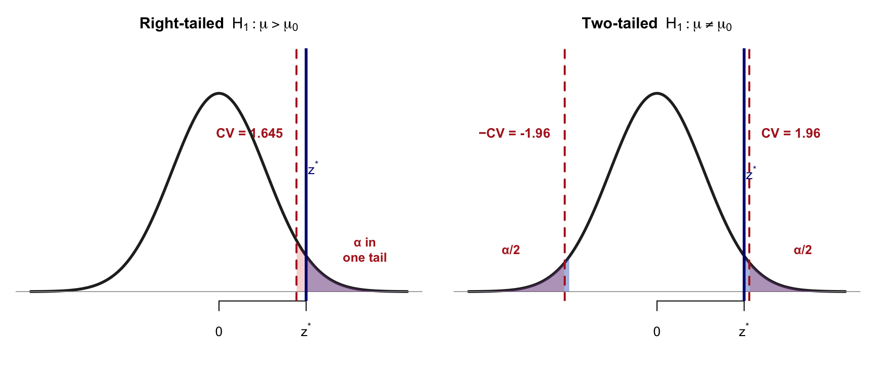
| 0.05 | 1.645 | 1.960 |
| 0.01 | 2.326 | 2.576 |
| 0.001 | 3.090 | 3.291 |
Logic, Geometry, and Decisions
Core question: Is our test statistic surprising if H₀ were true?
| Approach | What we locate | Decision rule |
|---|---|---|
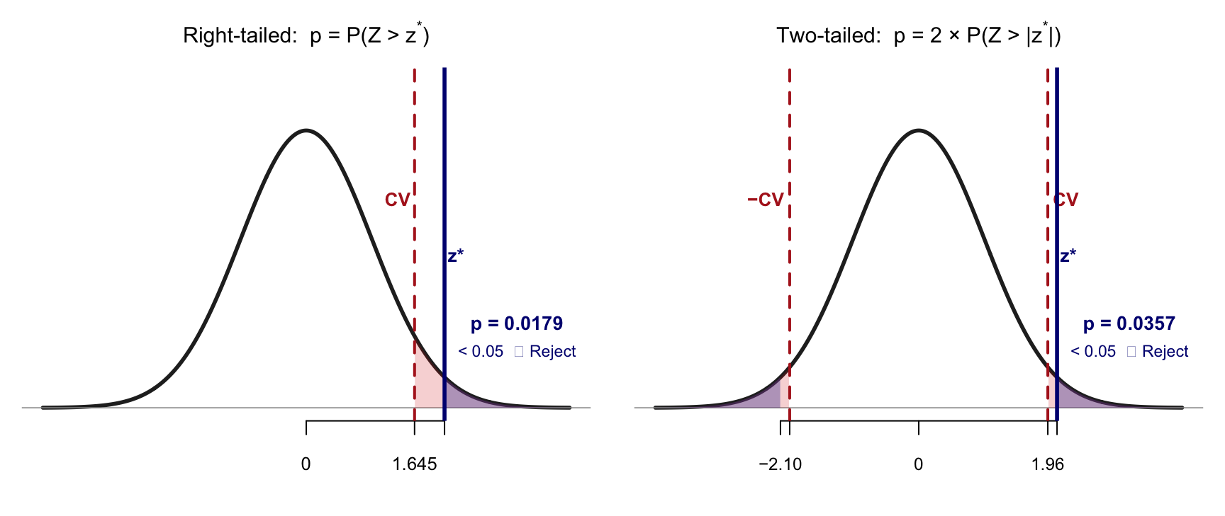
| P-value | Area in the tail(s) beyond the test statistic | Reject H₀ if p < α |
| Critical value | A threshold on the x-axis | Reject H₀ if the test statistic enters the rejection region |
Important
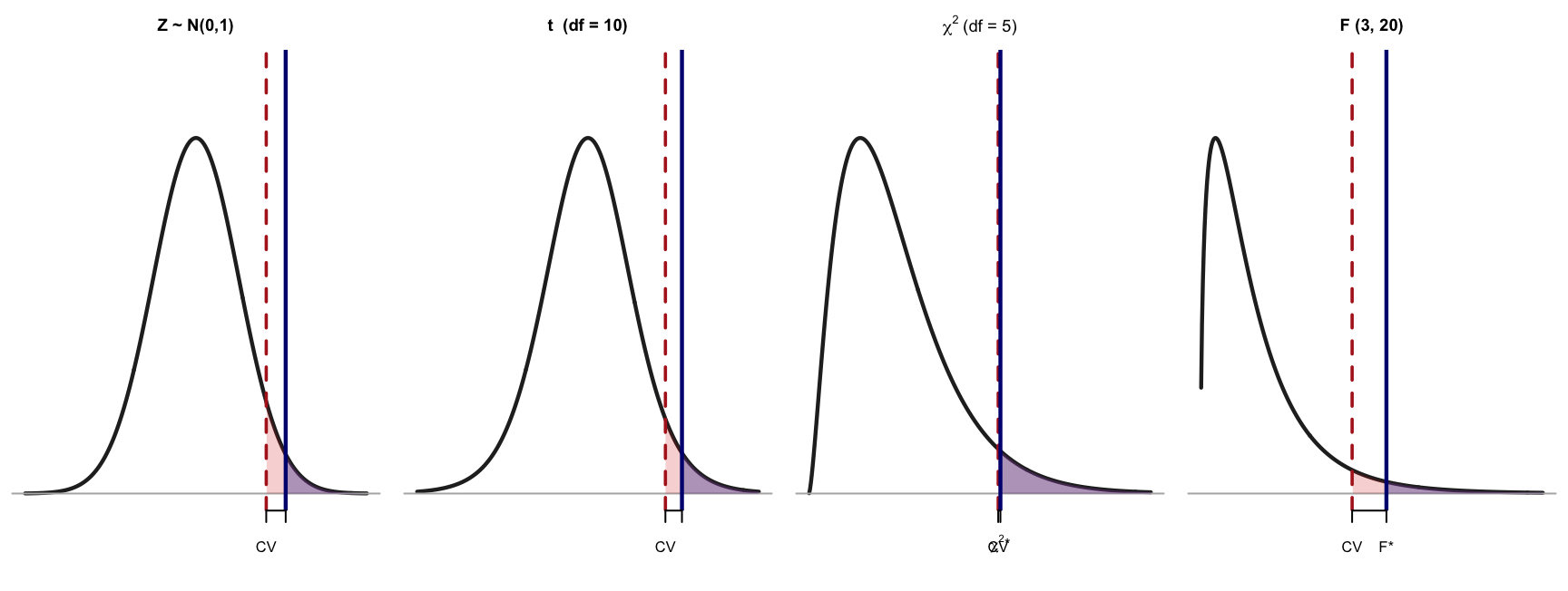
These two approaches are equivalent — they are two views of the same geometry.
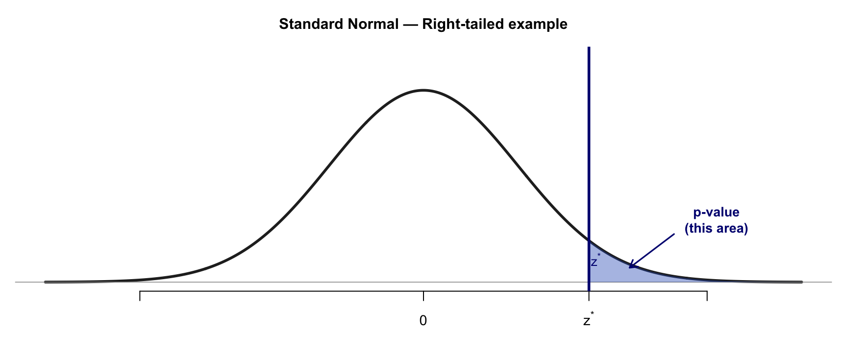
p-value = P(seeing something this extreme or more | H₀ is true)
The further z* moves into the tail → smaller area → smaller p-value → stronger evidence against H₀
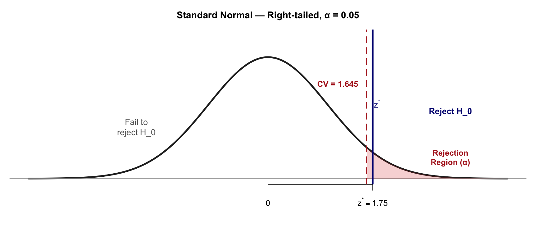
z* > CV → z* is inside the rejection region → Reject H₀
The CV cuts off exactly α in the tail; anything past it is “too extreme under H₀”
p-value area rejection region — test statistic (z*) – critical value (CV)
Key features: Symmetric around 0 · Ranges (−∞, +∞) · Area under curve = 1 · No parameters needed
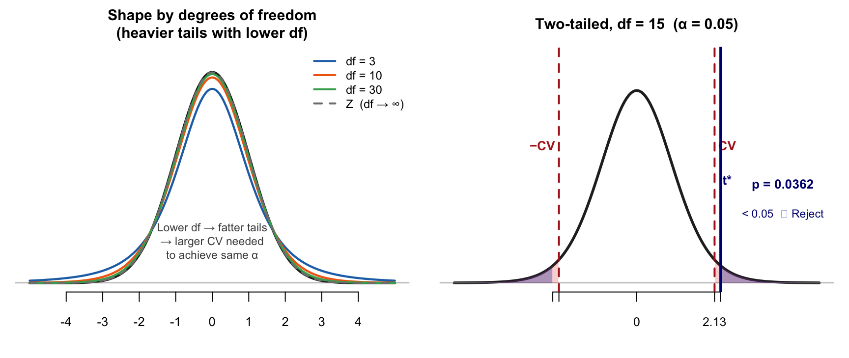
Key features: Symmetric around 0 · df controls tail weight · As df → ∞, t → Z · Always check df first — it changes the CV
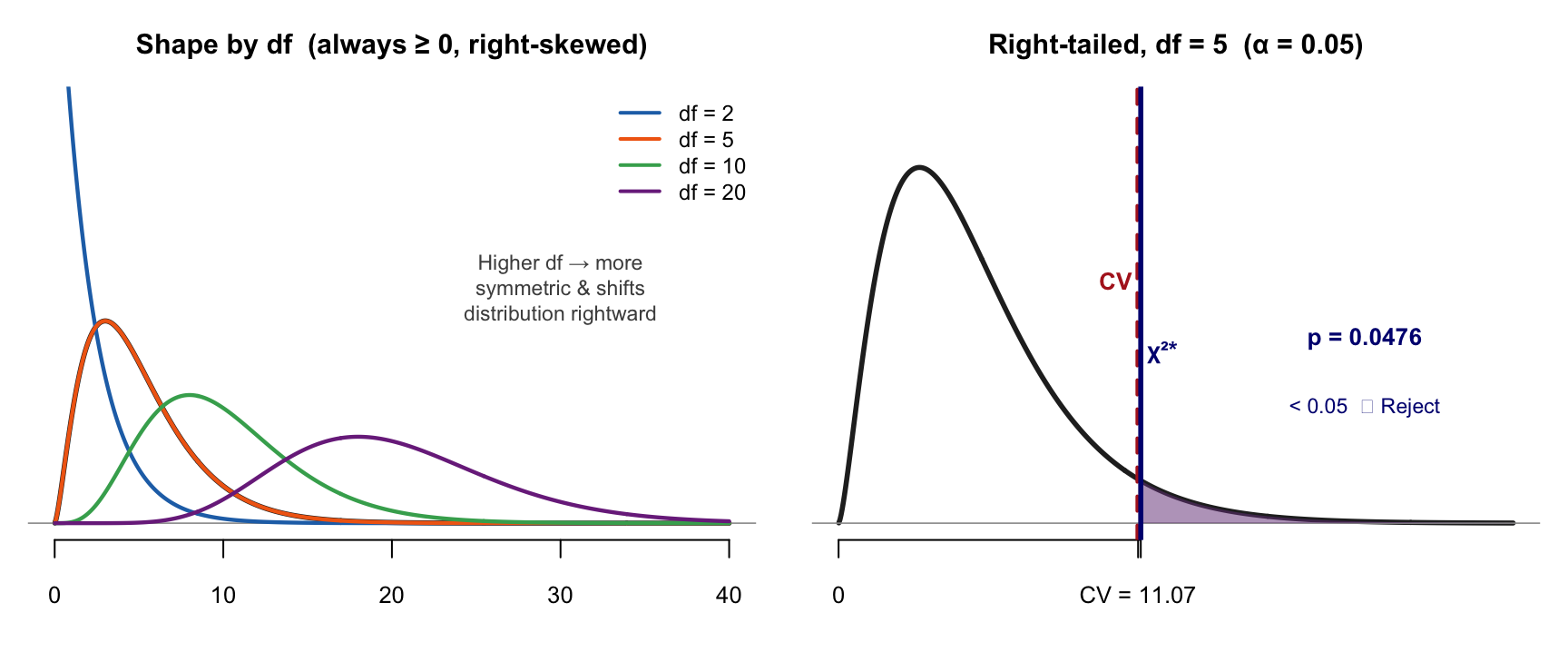
Key features: Values always ≥ 0 · Right-skewed · Only right-tail matters · Uses: goodness-of-fit, independence tests, variance tests
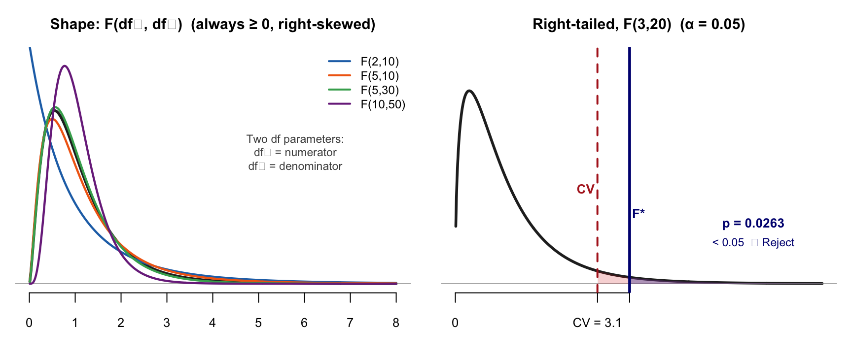
Key features: Values always ≥ 0 · Right-skewed · Two df parameters · Uses: ANOVA, overall regression F-test · F* = ratio of two variance estimates
| Distribution | Symmetric? | Range | Typical test direction | # of df |
|---|---|---|---|---|
| Z | ✓ | (−∞, +∞) | one or two-tailed | — |
| t | ✓ | (−∞, +∞) | one or two-tailed | 1 |
| χ² | ✗ | [0, +∞) | right-tailed | 1 |
| F | ✗ | [0, +∞) | right-tailed | 2 (df₁, df₂) |
Z — critical values
Values are the same regardless of sample size.
| α | One-tailed | Two-tailed |
|---|---|---|
| 0.10 | 1.282 | 1.645 |
| 0.05 | 1.645 | 1.960 |
| 0.01 | 2.326 | 2.576 |
| 0.001 | 3.090 | 3.291 |
t — critical values (two-tailed)
As df grows the t-distribution approaches Z; notice the bottom row matches the Z table.
| df | α = 0.10 (2-tail) | α = 0.05 (2-tail) | α = 0.01 (2-tail) |
|---|---|---|---|
| 5 | 2.015 | 2.571 | 4.032 |
| 10 | 1.812 | 2.228 | 3.169 |
| 15 | 1.753 | 2.131 | 2.947 |
| 20 | 1.725 | 2.086 | 2.845 |
| 30 | 1.697 | 2.042 | 2.750 |
| 60 | 1.671 | 2.000 | 2.660 |
| ∞ (→ Z) | 1.645 | 1.960 | 2.576 |
χ² — critical values (right-tailed)
| df | α = 0.10 | α = 0.05 | α = 0.025 | α = 0.01 |
|---|---|---|---|---|
| 1 | 2.706 | 3.841 | 5.024 | 6.635 |
| 2 | 4.605 | 5.991 | 7.378 | 9.210 |
| 3 | 6.251 | 7.815 | 9.348 | 11.345 |
| 4 | 7.779 | 9.488 | 11.143 | 13.277 |
| 5 | 9.236 | 11.070 | 12.833 | 15.086 |
| 10 | 15.987 | 18.307 | 20.483 | 23.209 |
| 15 | 22.307 | 24.996 | 27.488 | 30.578 |
| 20 | 28.412 | 31.410 | 34.170 | 37.566 |
F — critical values (right-tailed, α = 0.05)
| df₂ df₁ | df₁ = 1 | df₁ = 2 | df₁ = 3 | df₁ = 4 | df₁ = 5 |
|---|---|---|---|---|---|
| df₂ = 10 | 4.96 | 4.10 | 3.71 | 3.48 | 3.33 |
| df₂ = 15 | 4.54 | 3.68 | 3.29 | 3.06 | 2.90 |
| df₂ = 20 | 4.35 | 3.49 | 3.10 | 2.87 | 2.71 |
| df₂ = 30 | 4.17 | 3.32 | 2.92 | 2.69 | 2.53 |
| df₂ = 60 | 4.00 | 3.15 | 2.76 | 2.53 | 2.37 |
Note
For F, you need both df₁ (numerator) and df₂ (denominator). For χ² and t, only one df. For Z, no df at all.
The geometry is always the same
A smaller p-value ↔︎ a test statistic further in the tail ↔︎ further past the CV. Setting p-value = α gives you exactly the critical value: CV = F⁻¹(1 − α).