STAT 17: Statistical Methods for Business and Economics

Prof. Marcela Alfaro Cordoba

Statistics - UCSC

28 Apr 2026

Sarah’s Next Challenge 📊

Last time, Sarah discovered that the median watch time is 12 hours, while the mean is 18 hours…

But her manager asks: “How consistent are our users?”

Do most users watch similar amounts?
Or is there huge variation?
What does the “shape” of our data tell us?

The Problem: Measures of center don’t tell the whole story! 🤔

Today’s mission: Learn to measure and interpret data spread and distribution shape!

What We’ll Accomplish Today

By the end of this lecture, you will be able to:

✅ Calculate and interpret measures of spread (range, variance, standard deviation) using Google Sheets
✅ Understand the relationship between variance and standard deviation
✅ Identify and interpret skewness in distributions
✅ Recognize when data is symmetric, left-skewed, or right-skewed

Why Spread Matters 🎯

Two datasets with the same mean (15 hours):

Dataset A: 14, 14, 15, 15, 16, 16

Dataset B: 5, 8, 12, 18, 22, 25

Both have mean = 15 hours

But they look completely different!

Question: Which dataset represents more consistent user behavior?

Answer: Dataset A! The values are clustered tightly around the mean.

Visualizing Spread

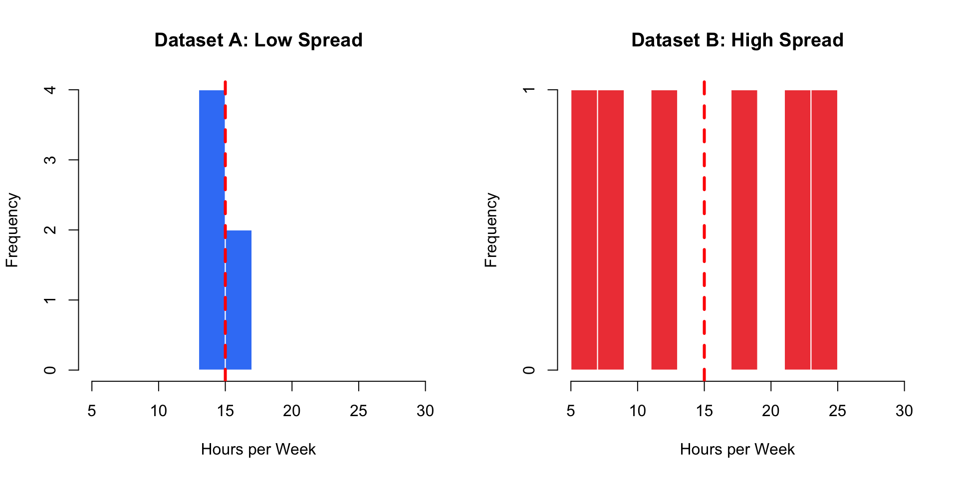
Red dashed line = Mean (15 hours for both)

Measures of Spread: Overview 📏

Three key measures:

Range - Difference between maximum and minimum values (simplest)
Variance - Average of squared deviations from the mean (foundation)
Standard Deviation - Square root of variance (most interpretable)

Each measure tells us how spread out or dispersed the data is!

The Range

Definition: Range = Maximum - Minimum

Example: Sarah’s watch times (hours)

Data: 5, 8, 10, 12, 15, 18, 95

Range = 95 - 5 = 90 hours

Pros:

✅ Very easy to calculate
✅ Quick sense of data spread

Cons:

❌ Uses only two values (ignores the rest!)
❌ Extremely sensitive to outliers

Range in Google Sheets

Example data in cells A1:A7: 5, 8, 10, 12, 15, 18, 95

Formula: =MAX(A1:A7) - MIN(A1:A7)

Result: 90

Alternative (more explicit):

In cell B1: =MAX(A1:A7)
In cell B2: =MIN(A1:A7)
In cell B3: =B1 - B2

Limitation: Notice how one outlier (95) drastically affects the range!

Deviation from the Mean 📊

To measure spread better, we need to consider how far each value is from the mean.

Deviation = (Value - Mean) = \(x_i - \bar{x}\)

Example: If mean = 12 hours

A user who watches 15 hours has deviation = 15 - 12 = +3
A user who watches 8 hours has deviation = 8 - 12 = -4

Positive deviation = above average
Negative deviation = below average

Why Not Just Average the Deviations?

Let’s try: Data = 5, 8, 10, 12, 15, 18, 95

Mean = (5+8+10+12+15+18+95)/7 = 23.3 hours

Deviations:

5 - 23.3 = -18.3
8 - 23.3 = -15.3
10 - 23.3 = -13.3
12 - 23.3 = -11.3
15 - 23.3 = -8.3
18 - 23.3 = -5.3
95 - 23.3 = +71.7

Sum of deviations = -18.3 - 15.3 - 13.3 - 11.3 - 8.3 - 5.3 + 71.7 = 0 😱

The Problem: Deviations Cancel Out!

Mathematical fact: \(\sum_{i=1}^{n} (x_i - \bar{x}) = 0\) always!

Why? Positive and negative deviations always cancel each other out.

Solution: Square the deviations to make them all positive!

\((x_i - \bar{x})^2\) is always positive (or zero)

Variance: The Foundation

Definition: The average of the squared deviations from the mean

Sample Variance: \(s^2 = \frac{\sum_{i=1}^{n} (x_i - \bar{x})^2}{n-1}\)

Population Variance: \(\sigma^2 = \frac{\sum_{i=1}^{N} (x_i - \mu)^2}{N}\)

Key differences:

Sample: Divide by (n-1) - called “degrees of freedom”
Population: Divide by N
We usually work with samples, so use n-1!

Why n-1 Instead of n? 🤔

Short answer: To get an unbiased estimate of population variance.

Intuition: When we calculate \(\bar{x}\) from the sample, we “use up” one degree of freedom. Only (n-1) values are truly “free” to vary.

For this class: Just remember to use n-1 for sample variance!

Good news: Google Sheets handles this automatically! 🎉

Calculating Variance: Step by Step

Example: Dataset A = 14, 14, 15, 15, 16, 16 (n = 6)

Step 1: Calculate mean

\(\bar{x} = \frac{14+14+15+15+16+16}{6} = 15\) hours

Step 2: Calculate each squared deviation

\((14-15)^2 = 1\)
\((14-15)^2 = 1\)
\((15-15)^2 = 0\)
\((15-15)^2 = 0\)
\((16-15)^2 = 1\)
\((16-15)^2 = 1\)

Calculating Variance: Step by Step (cont.)

Step 3: Sum the squared deviations

\(\sum (x_i - \bar{x})^2 = 1 + 1 + 0 + 0 + 1 + 1 = 4\)

Step 4: Divide by n-1

\(s^2 = \frac{4}{6-1} = \frac{4}{5} = 0.8\) hours²

Units: Variance is in squared units (hours²) - not very intuitive! 🤔

Variance in Google Sheets

Example data in A1:A6: 14, 14, 15, 15, 16, 16

Formula: =VAR.S(A1:A6)

Result: 0.8

Alternative functions:

=VAR.S(range) - Sample variance (use this for samples!)
=VAR.P(range) - Population variance (rarely used)
=VAR(range) - Older function (same as VAR.S)

Remember: The “S” stands for “Sample” (divides by n-1)!

Standard Deviation: Most Useful!

Definition: The square root of the variance

Sample Standard Deviation: \(s = \sqrt{s^2} = \sqrt{\frac{\sum_{i=1}^{n} (x_i - \bar{x})^2}{n-1}}\)

Population Standard Deviation: \(\sigma = \sqrt{\sigma^2}\)

Why take the square root?

To get back to the original units! 🎯

Standard Deviation Example

Dataset A: Variance = 0.8 hours²

Standard Deviation: \(s = \sqrt{0.8} \approx 0.89\) hours

Interpretation: On average, users’ watch times deviate from the mean by about 0.89 hours (or 53 minutes).

Much more interpretable than “0.8 hours²”! ✅

Standard Deviation in Google Sheets

Example data in A1:A6: 14, 14, 15, 15, 16, 16

Formula: =STDEV.S(A1:A6)

Result: ≈ 0.89

Alternative functions:

=STDEV.S(range) - Sample standard deviation (use this!)
=STDEV.P(range) - Population standard deviation
=STDEV(range) - Older function (same as STDEV.S)

Pro tip: You can also use =SQRT(VAR.S(A1:A6)) - gives the same result!

Comparing Datasets with Standard Deviation

Dataset A: 14, 14, 15, 15, 16, 16

Mean = 15 hours
SD ≈ 0.89 hours (low spread)

Dataset B: 5, 8, 12, 18, 22, 25

Mean = 15 hours
SD ≈ 7.58 hours (high spread)

Interpretation: Dataset B has users with much more variable viewing habits!

Calculating SD for Dataset B

Dataset B: 5, 8, 12, 18, 22, 25 (n = 6, mean = 15)

Squared deviations:

\((5-15)^2 = 100\)
\((8-15)^2 = 49\)
\((12-15)^2 = 9\)
\((18-15)^2 = 9\)
\((22-15)^2 = 49\)
\((25-15)^2 = 100\)

\(\sum (x_i - \bar{x})^2 = 316\)

\(s^2 = \frac{316}{5} = 63.2\) hours²

\(s = \sqrt{63.2} \approx 7.95\) hours ✅

🧘‍♀️ STRETCH BREAK

Time to move! (5 minutes)

Stand up and stretch 🤸‍♀️
Chat with neighbors 💬
Grab some water 💧

When we return: Distribution shape

Understanding Distribution Shape 📊

Spread tells us how dispersed data is, but SHAPE tells us how it’s distributed!

Three main shapes:

Symmetric - balanced on both sides
Right-skewed (positively skewed) - tail extends right
Left-skewed (negatively skewed) - tail extends left

Symmetric Distribution

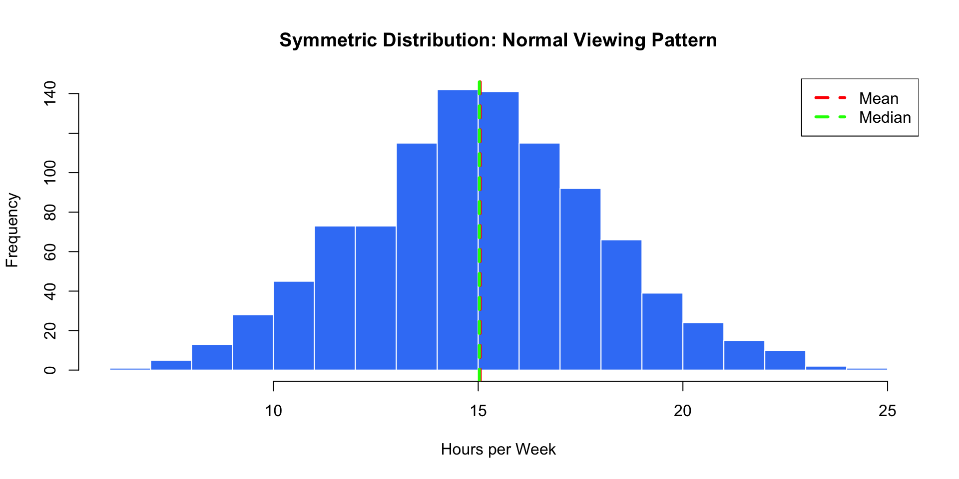
Key feature: Mean ≈ Median (they overlap!)

Right-Skewed Distribution (Positive Skew)

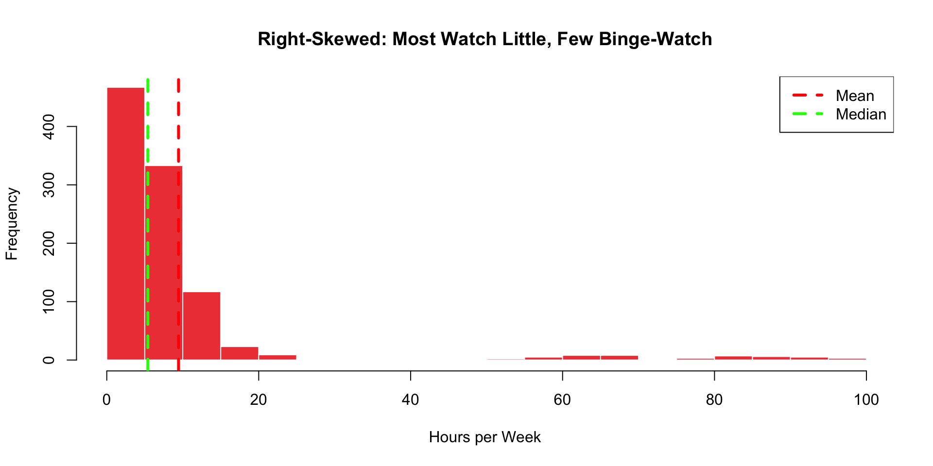
Key feature: Mean > Median (pulled by outliers on the right!)

Right-Skewed: Real Netflix Example

Sarah’s actual data (first 20 users, hours per week):

5, 6, 7, 8, 8, 9, 10, 10, 11, 12, 13, 14, 15, 18, 20, 22, 45, 67, 82, 95

Calculate in Google Sheets:

Mean = =AVERAGE(A1:A20) = 21.85 hours
Median = =MEDIAN(A1:A20) = 11.5 hours

Mean > Median → Right-skewed!

The extreme binge-watchers (45, 67, 82, 95) pull the mean up!

Left-Skewed Distribution (Negative Skew)

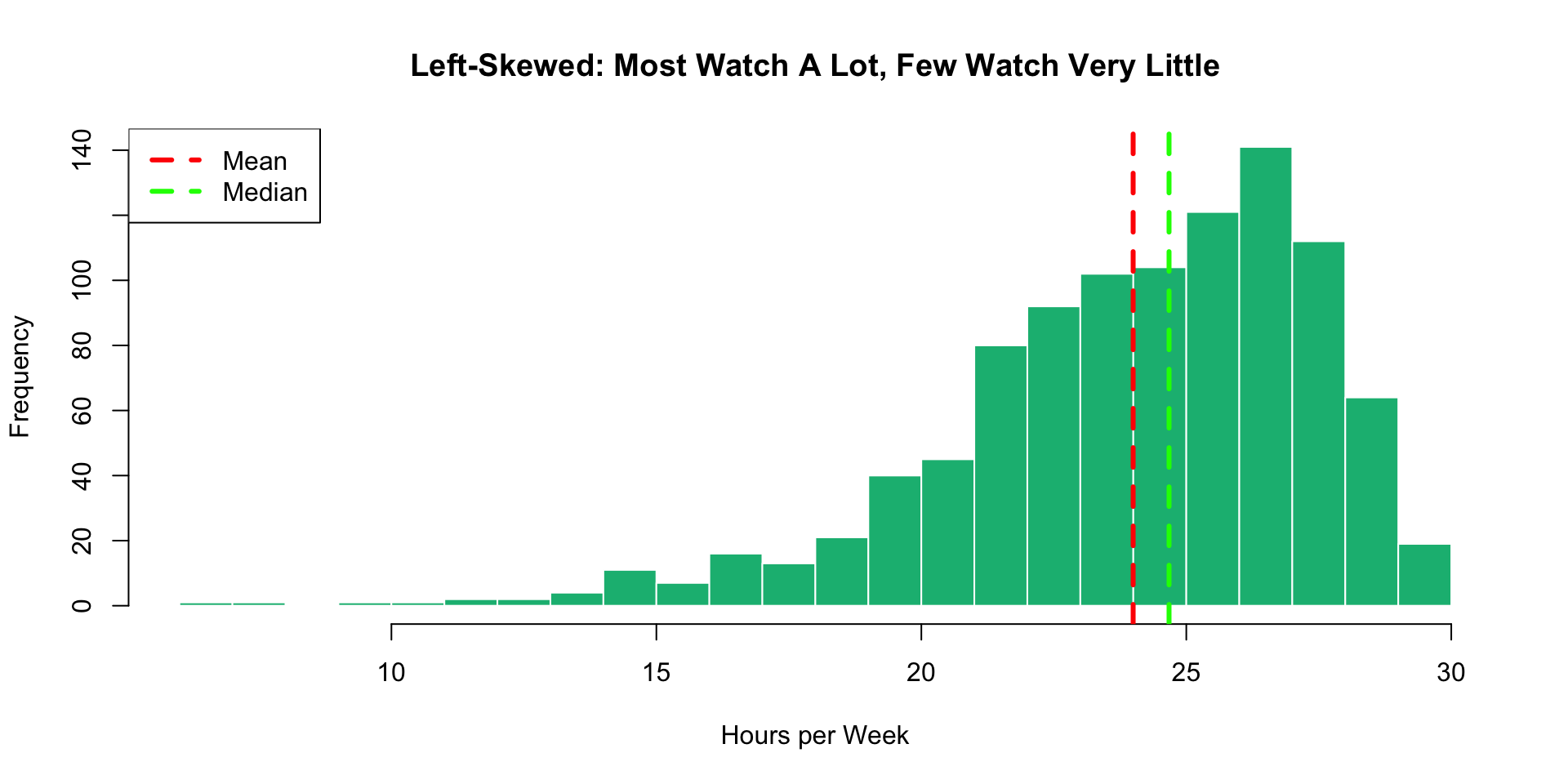
Key feature: Mean < Median (pulled by low outliers on the left!)

Identifying Skewness: The Rules 🎯

Three-step process:

Calculate mean and median in Google Sheets
Compare their values
Determine skewness:
- If Mean ≈ Median → Symmetric
- If Mean > Median → Right-skewed (tail extends right)
- If Mean < Median → Left-skewed (tail extends left)

Pro tip: Look at a histogram too - visual confirmation helps! 📊

Why Skewness Matters 💡

For Sarah’s Netflix analysis:

Right-skewed watch times tell her:

Most users are casual viewers (10-15 hours/week)
A small group of super-users (50+ hours/week)
Should report median (more representative)
Target different strategies for casual vs. super-users

Business impact:

✅ Retention campaigns for super-users
✅ Engagement campaigns for casual users
✅ Realistic expectations for “typical” usage

Real-World Skewed Distributions

Right-skewed examples (Mean > Median):

Income distributions (few billionaires pull mean up)
House prices (luxury homes pull mean up)
Website traffic (viral posts pull mean up)
Netflix watch times (binge-watchers pull mean up)

Left-skewed examples (Mean < Median):

Test scores with many high achievers
Age at retirement (most retire around 65, few retire early)
Product ratings on Amazon (most are 4-5 stars)

Visualizing Skewness in Google Sheets

Steps to check for skewness:

Enter your data in column A
Calculate measures:
- In B1: =AVERAGE(A:A) (mean)
- In B2: =MEDIAN(A:A) (median)
- In B3: =STDEV.S(A:A) (standard deviation)
Create histogram: Insert → Chart → Histogram
Compare mean vs median
Examine the histogram shape

The Complete Picture: Spread + Shape

To fully describe a dataset, Sarah needs BOTH:

Measures of Center:

Mean
Median
Mode

Where is the data centered?

Measures of Spread:

Range
Variance
Standard deviation

How dispersed is the data?

Plus Shape:

Symmetric, right-skewed, or left-skewed?
Where are the outliers?

Sarah’s Complete Analysis 🎉

Weekly Watch Time Data (hours):

Measures of Center:

Mean = 18 hours
Median = 12 hours
Mode = 10 hours

Measures of Spread:

Range = 90 hours
Standard deviation = 15.3 hours

Distribution Shape:

Right-skewed (Mean > Median)
Most users: 8-15 hours
Extreme users: 50-95 hours

Sarah’s Recommendation to Executives 📋

“Based on my analysis…”

Center: “The median viewing time is 12 hours per week, which better represents our typical user than the mean (18 hours), since we have some extreme binge-watchers.”

Spread: “There’s substantial variation in viewing habits (SD = 15.3 hours), indicating diverse user segments.”

Shape: “Our distribution is right-skewed, with most users watching 8-15 hours, but a valuable segment watching 50+ hours weekly.”

Action: “We should create targeted strategies for both casual viewers and super-users!”

Google Sheets Function Summary 💻

Essential Functions for Spread & Shape:

Function	Purpose	Example
`=MAX(range)`	Maximum value	`=MAX(A1:A100)`
`=MIN(range)`	Minimum value	`=MIN(A1:A100)`
`=VAR.S(range)`	Sample variance	`=VAR.S(A1:A100)`
`=STDEV.S(range)`	Sample std dev	`=STDEV.S(A1:A100)`
`=AVERAGE(range)`	Mean	`=AVERAGE(A1:A100)`
`=MEDIAN(range)`	Median	`=MEDIAN(A1:A100)`

Remember: Use .S versions for samples (which is almost always!)

Your Expanded Statistical Toolkit 🧰

Measures of Spread:

Range = Max - Min (simple but sensitive to outliers)
Variance = Average of squared deviations (in squared units)
Standard Deviation = √Variance (most interpretable!)

Distribution Shape:

Symmetric: Mean ≈ Median
Right-skewed: Mean > Median (tail extends right)
Left-skewed: Mean < Median (tail extends left)

Google Sheets Mastery:

Use STDEV.S() and VAR.S() for samples
Compare mean vs median to detect skewness
Create histograms to visualize shape

Common Mistakes to Avoid ⚠️

Using VAR.P or STDEV.P for sample data (almost always use .S versions!)
Ignoring outliers when interpreting mean and standard deviation
Forgetting units - variance is in squared units, SD is in original units
Confusing skew direction - “right-skewed” means tail extends RIGHT (mean pulled right)
Relying only on center - always report spread and shape too!

Quick Practice: What’s the Skewness? 🤔

Without calculating, predict the skewness:

Scenario 1: Ages of US residents

Most people in middle age ranges, fewer children and elderly

Answer: Approximately symmetric (slight variations)

Scenario 2: Incomes in the United States

Most people earn moderate incomes, few earn millions

Answer: Right-skewed! (Mean > Median)

Scenario 3: Scores on an easy exam

Most students score 80-100, few score below 70

Answer: Left-skewed! (Mean < Median)

Looking Ahead

Next Class: Introduction to Probability

Understanding randomness
Basic probability rules
Applying probability to real data

This week’s WS and HW: Will include analyzing a dataset using everything we’ve learned - center, spread, and shape! 📊

Questions? Office hours are the perfect place to practice these calculations! 🤗

Quick Knowledge Check ✅

Rate your confidence (1-5) on Ed Discussion:

Calculating range, variance, and standard deviation in Google Sheets ⭐⭐⭐⭐⭐
Understanding why we use n-1 for sample variance ⭐⭐⭐⭐⭐
Interpreting standard deviation in context ⭐⭐⭐⭐⭐
Identifying skewness by comparing mean and median ⭐⭐⭐⭐⭐
Recognizing skewed distributions in histograms ⭐⭐⭐⭐⭐

If you rated anything 3 or below, please visit office hours! 🤝

Thank you! 📊✨

Questions? Office hours information on Canvas.

Next up: Introduction to Probability & Statistical Thinking!