STAT 17: Linear Regression Part II
Statistics - UCSC
02 Dec 2025
📊 Case Study: TechStart Ventures (Continued)
The Next Challenge
Last time, we found: - Strong correlation (r = 0.85) between advertising and revenue - Regression equation: \(\widehat{\text{Revenue}} = 12.45 + 0.78 \times \text{Advertising}\)
But the investors ask:
- Is this relationship statistically significant? Or could it be due to chance?
- How confident can we be in our predictions?
- Could the true slope actually be zero in the population?
- What’s the margin of error for our revenue forecasts?
Today: Move from description to inference - test hypotheses and quantify uncertainty!
Learning Objectives 🎯
By the end of today’s lecture, you will be able to:
- Understand the assumptions/conditions for regression inference
- Test hypotheses about the population slope (\(\beta_1\))
- Interpret p-values and t-statistics in regression
- Calculate and interpret confidence intervals for slope
- Understand standard error of regression
- Assess statistical significance of relationships
- Use Google Sheets for regression inference
Review: What We Know So Far
Sample Statistics (Descriptive)
- Sample correlation: \(r = 0.85\)
- Sample slope: \(b_1 = 0.78\)
- Sample intercept: \(b_0 = 12.45\)
- Sample R²: \(R^2 = 0.72\)
These describe our sample data
Population Parameters (Inferential)
- Population correlation: \(\rho\) (rho)
- Population slope: \(\beta_1\) (beta)
- Population intercept: \(\beta_0\) (beta)
- Population R²: not typically estimated
These are the true values we want to know
Important
Key Question: Can we use our sample statistics to make inferences about population parameters?
The Sampling Distribution of \(b_1\)
If we took many different samples and calculated \(b_1\) each time:
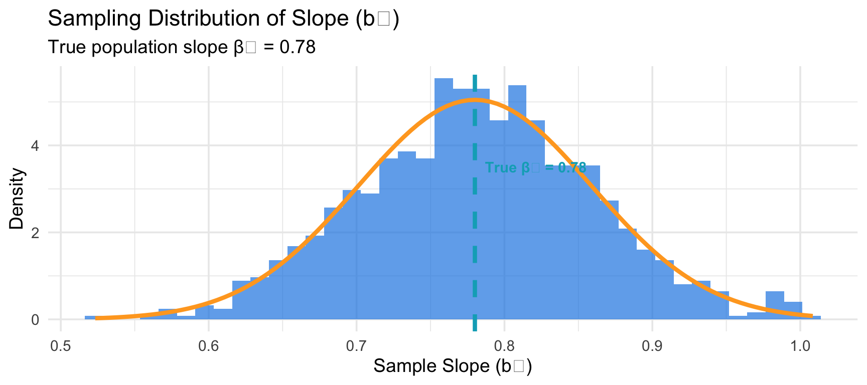
Key insight: \(b_1\) varies from sample to sample, but centers around the true \(\beta_1\)!
Conditions for Regression Inference
Before doing inference, check these conditions:
- Linearity: Relationship between x and y is linear
- Check: Scatterplot shows linear pattern
- Independence: Observations are independent
- Check: Random sampling, no time series
- Normality: Residuals are approximately normally distributed
- Check: Histogram or normal probability plot of residuals
- Less important with large samples (n > 30)
- Equal variance (Homoscedasticity): Spread of residuals is constant
- Check: Residual plot shows no fan/cone shape
Warning
Mnemonic: LINE (Linearity, Independence, Normality, Equal variance)
Checking Conditions: Residual Plot
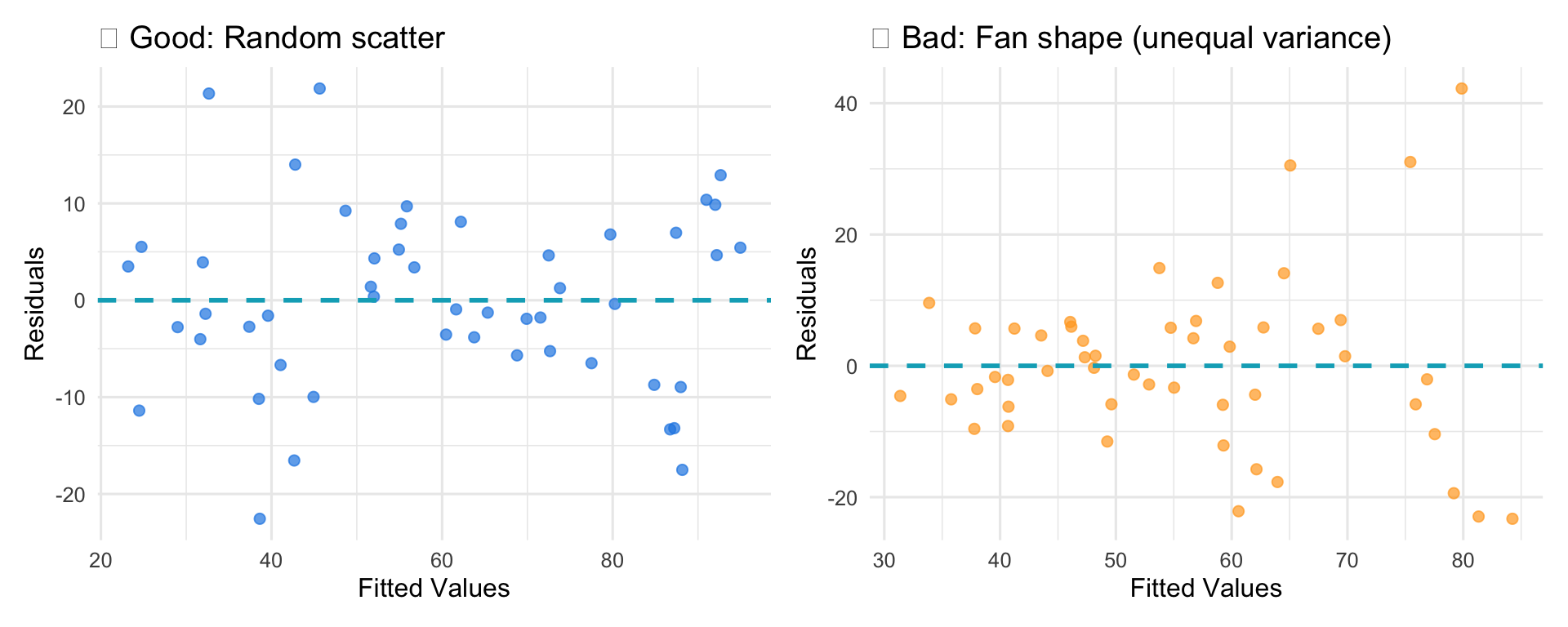
What to look for:
- Good: Random scatter around zero, no patterns
- Bad: Fan/cone shape, curves, clusters
THINK-PAIR-SHARE 1 (5 minutes)
Which condition is MOST important to check before regression inference?
A. The residuals are perfectly normal
B. The relationship is linear
C. Every single data point is independent
D. R² is above 0.70

Part 1: Testing Hypotheses About Slope
Is the relationship statistically significant?
Hypothesis Test for Slope (\(\beta_1\))
Standard Test Setup
Hypotheses: \[H_0: \beta_1 = 0\] (No linear relationship in population) \[H_a: \beta_1 \neq 0\] (Linear relationship exists)
Test Statistic: \[t = \frac{b_1 - 0}{SE_{b_1}}\]
where \(SE_{b_1}\) is the standard error of the slope
Degrees of freedom: \(df = n - 2\)
For TechStart: With n = 25 startups, df = 23
Understanding Standard Error of Slope
Standard Error (\(SE_{b_1}\)): Measures variability of slope estimates across samples
\[SE_{b_1} = \frac{s_e}{s_x \sqrt{n-1}}\]
where:
- \(s_e\) = standard error of the regression (residual standard error)
- \(s_x\) = standard deviation of x
- \(n\) = sample size
What affects \(SE_{b_1}\)?
Decreases when: - Residuals are smaller (\(s_e\) ↓) - X has more spread (\(s_x\) ↑) - Sample size is larger (\(n\) ↑)
Result: More precise slope estimate!
TechStart Example: Testing Significance
Given regression output from Google Sheets:
- Sample slope: \(b_1 = 0.78\)
- Standard error: \(SE_{b_1} = 0.12\)
- n = 25 startups
Calculate t-statistic:
\[t = \frac{b_1 - 0}{SE_{b_1}} = \frac{0.78 - 0}{0.12} = 6.50\]
Find p-value: With df = 23, using t-table or Sheets: p-value < 0.001
Decision: Reject \(H_0\) at α = 0.05
Conclusion: There is strong evidence of a significant positive linear relationship between advertising and revenue in the population (t = 6.50, p < 0.001).
Interpreting P-values in Regression
P-value: Probability of getting a slope as extreme as ours (or more) if true slope is zero
Small p-value (< \(\alpha\))
- Statistical evidence against \(H_0\)
- Relationship is statistically significant
- Slope is likely NOT zero
- Can use model for prediction
TechStart: p < 0.001
→ Statistical evidence!
Large p-value (≥ \(\alpha\))
- Weak evidence against \(H_0\)
- Relationship is not statistically significant
- Can’t rule out zero slope
- Be cautious about predictions
Example: p = 0.23
→ Not significant
Warning
Statistical significance ≠ Practical significance!
THINK-PAIR-SHARE 2 (5 minutes)
Regression output shows: \(b_1 = 0.45\), \(SE_{b_1} = 0.30\), p-value = 0.15
What should we conclude at α = 0.05?
A. The relationship is statistically significant
B. The relationship is not statistically significant
C. We need more data to decide
D. The slope is definitely zero
Part 2: Confidence Intervals for Slope
Quantifying Uncertainty
Confidence Interval for \(\beta_1\)
Formula
\[b_1 \pm t^* \times SE_{b_1}\]
where:
- \(b_1\) = sample slope
- \(t^*\) = critical value from t-distribution with df = n - 2
- \(SE_{b_1}\) = standard error of slope
For TechStart (95% CI with df = 23):
- \(b_1 = 0.78\), \(SE_{b_1} = 0.12\)
- \(t^* = 2.069\) (from t-table)
\[0.78 \pm 2.069(0.12) = 0.78 \pm 0.25 = (0.53, 1.03)\]
Interpretation: We are 95% confident that for each additional $1,000 in advertising, revenue increases between $530 and $1,030 in the population.
Confidence Intervals and Hypothesis Tests
Important Connection
For a two-tailed test at significance level α:
If the \((1-\alpha) \times 100\%\) confidence interval for \(\beta_1\):
- Does NOT contain 0 → Reject \(H_0\) (statistically significant relationship)
- Contains 0 → Fail to reject \(H_0\) (not significant)
TechStart example:
- 95% CI: (0.53, 1.03)
- Does NOT contain 0
- Therefore: Reject \(H_0\) at α = 0.05 ✓
This provides more information than hypothesis test alone!
🍵 Break Time!
10 Minute Break
We’ll return to discuss standard error, confidence intervals for predictions, and Google Sheets implementation!
Part 3: Standard Error and Prediction Intervals
Quantifying Prediction Uncertainty
Standard Error of the Regression (\(s_e\))
Measures typical size of prediction errors (residuals)
\[s_e = \sqrt{\frac{\sum(y_i - \widehat{y}_i)^2}{n-2}} = \sqrt{\frac{\text{Sum of Squared Residuals}}{df}}\]
For TechStart
\(s_e = 9.8\) thousand dollars
Interpretation: Predictions are typically off by about $9,800, either direction
Also called:
- Residual standard error
- Standard error of the estimate
- Root Mean Square Error (RMSE)
Two Types of Intervals
Confidence Interval for Mean Response
Question: What’s the average y for a given x?
Example: What’s the average revenue for ALL startups spending $50k on ads?
Formula: \[\widehat{y} \pm t^* \times SE_{\text{mean}}\]
Narrower interval
(more precise)
Prediction Interval for Individual Response
Question: What y will we observe for a new case?
Example: What revenue will THIS specific startup with $50k ad spending achieve?
Formula: \[\widehat{y} \pm t^* \times SE_{\text{pred}}\]
Wider interval
(more uncertainty)
Prediction Interval Example
Predict revenue for a startup spending $50,000 on advertising:
Point estimate: \[\widehat{\text{Revenue}} = 12.45 + 0.78(50) = 51.45 \text{ thousand}\]
95% Prediction Interval: (30.8, 72.1) thousand
Interpretation: We are 95% confident this specific startup will generate between $30,800 and $72,100 in revenue.
Note: Wide interval reflects uncertainty in predicting individual cases!
Warning
Key Business Insight: Even with strong correlation (r = 0.85), individual predictions have substantial uncertainty. Don’t over-rely on point estimates!
THINK-PAIR-SHARE 3 (5 minutes)
Why is a prediction interval wider than a confidence interval at the same x value?
A. Because we use a larger t* value
B. Because it accounts for both estimation uncertainty AND individual variation
C. Because the sample size is smaller
D. Because predictions are less accurate
Reading Regression Output
Example output for TechStart:
| Coefficient | Estimate | Std Error | t-stat | p-value |
|---|---|---|---|---|
| Intercept | 12.45 | 3.82 | 3.26 | 0.004 |
| Advertising | 0.78 | 0.12 | 6.50 | < 0.001 |
Additional statistics:
- R² = 0.72
- \(s_e\) = 9.8
- df = 23
What this tells us:
- Both intercept and slope are statistically significant (p < 0.05)
- Advertising coefficient: \(b_1 = 0.78 \pm 2.069(0.12)\) → 95% CI: (0.53, 1.03)
- Model explains 72% of variance
- Typical prediction error: $9,800
Complete Inference Example
TechStart Ventures: Full Analysis
Research Question: Is advertising spending significantly related to revenue?
1. Check Conditions: - ✓ Linearity: Scatterplot shows linear pattern - ✓ Independence: Random sample of startups - ✓ Normality: Residuals approximately normal (n = 25) - ✓ Equal variance: No fan shape in residual plot
2. Hypothesis Test: - \(H_0: \beta_1 = 0\) vs \(H_a: \beta_1 \neq 0\) - Test statistic: t = 6.50, df = 23 - p-value < 0.001 - Conclusion: Statistical evidence of significant relationship
3. Confidence Interval: - 95% CI for \(\beta_1\): (0.53, 1.03) - Interpretation: Each $1,000 increase in advertising increases revenue by $530-$1,030
4. Prediction: - For $50k advertising: \(\widehat{y}\) = 51.45k - 95% PI: (30.8, 72.1)k
THINK-PAIR-SHARE 4 (5 minutes)
Regression output shows p-value = 0.001 for slope. What does this mean?
A. There’s a 0.1% chance the null hypothesis is true
B. If there’s no relationship in the population, there’s a 0.1% chance of getting our result or more extreme
C. The slope is definitely not zero
D. 99.9% of the variance is explained
Statistical vs. Practical Significance
Important Distinction
Statistically Significant (p < α)
- Means: Effect likely exists in population (not just chance) - Determined by: Sample size, effect size, variability
Practically Significant
- Means: Effect is large enough to matter in practice - Determined by: Context, costs, benefits, business impact
Example scenarios:
| Scenario | Statistical | Practical | What to do? |
|---|---|---|---|
| Huge sample, tiny slope | Significant | Not significant | Don’t implement |
| Small sample, large slope | Not significant | Would be significant | Collect more data |
| Large sample, moderate slope | Significant | Significant | Implement! |
Key Concepts to Remember
Conditions (LINE): Must check before inference
- Linearity, Independence, Normality, Equal variance
Hypothesis test for slope: Tests if \(\beta_1 \neq 0\)
- Use t-statistic with df = n - 2
- Small p-value → significant relationship
Confidence interval for \(\beta_1\): Range of plausible values
- If doesn’t contain 0 → significant
- More informative than hypothesis test alone
Standard error (\(s_e\)): Typical prediction error
Prediction interval: Accounts for individual variation
- Wider than confidence interval
- Essential for business forecasting
Looking Ahead: Part III Preview
Next Time: Multiple Regression
- Predicting with multiple explanatory variables
- Example: Revenue = f(Advertising, Employees, Market Size)
- Interpreting coefficients in multiple regression
- R² vs Adjusted R²
- Which variables matter most?
The Power of Multiple Regression
Most real business problems involve multiple factors. Next time we’ll see how to model them simultaneously!
Questions? 💭
What questions do you have about:
- Conditions for inference?
- Hypothesis testing for slope?
- Confidence intervals?
- Prediction intervals?
- Interpreting regression output?
Thank You! 🎉
See you next time for:
Multiple Regression
Office hours: I’m available now if you have any questions
STAT 17 – Fall 2025