Stat 17: Introduction to Statistical Methods for Business and Economics

📊 Case Study: TechStart Ventures

The Challenge

TechStart Ventures is a venture capital firm evaluating startup investments. They’ve noticed that advertising spending seems related to revenue, but they need a systematic way to:

Quantify the strength of relationships between variables
Predict future revenue based on planned advertising budgets
Make decisions about which startups show the strongest revenue-to-marketing relationships

Today: Learn how correlation and linear regression can transform scattered data points into actionable business insights!

Learning Objectives 🎯

By the end of today’s lecture, you will be able to:

Understand and interpret scatterplots to visualize relationships
Calculate and interpret the correlation coefficient (r)
Develop and interpret simple linear regression equations
Understand what regression coefficients (slope and intercept) mean
Make predictions using regression equations
Use Google Sheets for correlation and regression analysis

Why Linear Regression is Essential

📈 Descriptive Statistics

Summarize relationships: How strong is the association between advertising and revenue?

Quantify direction: Does the relationship increase or decrease?

Visualize patterns: See trends in your data clearly

🔮 Inferential Statistics

Make predictions: Forecast revenue for new advertising budgets

Test hypotheses: Is this relationship statistically significant?

Quantify uncertainty: How confident are we in our predictions?

Important

Regression is the bridge between description and prediction!

Part 1: Visualizing Relationships 📉

Scatterplots

Guess the correlation: https://www.geogebra.org/m/KE6JfuF9

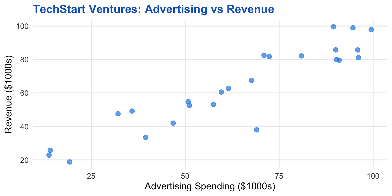
Scatterplots: The Foundation

What to look for:

Direction: Positive or negative?
Form: Linear or curved?
Strength: Tight cluster or scattered?
Outliers: Unusual points?

THINK-PAIR-SHARE 1 (5 minutes)

Looking at the scatterplot on the previous slide:

What best describes the relationship between advertising and revenue?

A. Strong positive linear relationship
B. Weak positive linear relationship
C. No relationship
D. Negative linear relationship

Part 2: Quantifying Relationships 📏

The Correlation Coefficient

Correlation Coefficient (r)

Measures the strength and direction of a linear relationship

Formula (you won’t calculate by hand!)

\[r = \frac{\sum (x_i - \bar{x})(y_i - \bar{y})}{\sqrt{\sum(x_i - \bar{x})^2 \sum(y_i - \bar{y})^2}}\]

Range: $-1 \leq r \leq +1$

Interpretation Guidelines:

Value of \|r\|	Strength
0.0 - 0.3	Weak
0.3 - 0.7	Moderate
0.7 - 1.0	Strong

For TechStart data: $r = 0.85$ → Strong positive linear relationship!

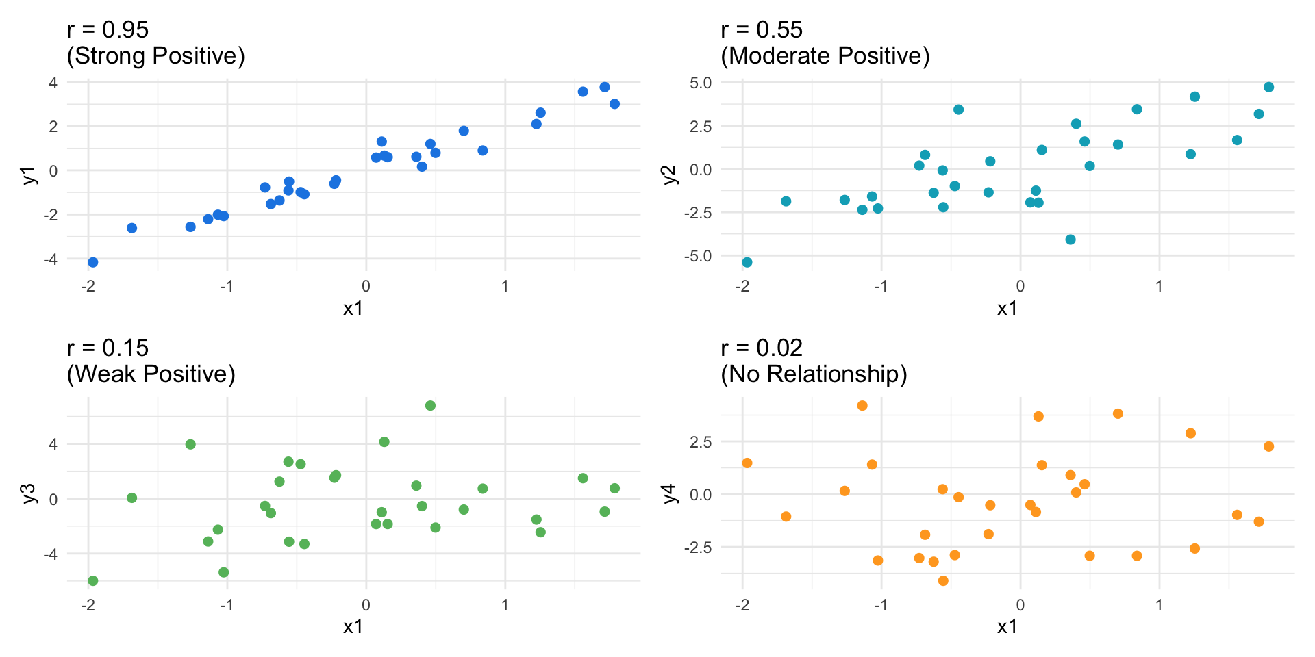
Understanding Correlation Values

Warning

⚠️ Correlation ≠ Causation! High correlation doesn’t mean one variable causes the other.

Google Sheets: Calculating Correlation

Function: =CORREL(range1, range2)

Example for TechStart data:

=CORREL(A2:A26, B2:B26)

Where: - A2:A26 contains Advertising data - B2:B26 contains Revenue data

Try it yourself!

Make your own copy of this sheet
Use =CORREL(A:A, B:B) for entire columns
Interpret the result using the guidelines

THINK-PAIR-SHARE 2 (7 minutes)

A study finds r = -0.68 between hours of study and test anxiety.

What does this mean?

A. More study causes less anxiety
B. Less study causes more anxiety
C. There’s a moderate negative relationship
D. There’s no relationship

🍵 Break Time!

5 Minute Break

We’ll return to build regression equations and make predictions!

Part 3: Simple Linear Regression 📐

Building Prediction Equations

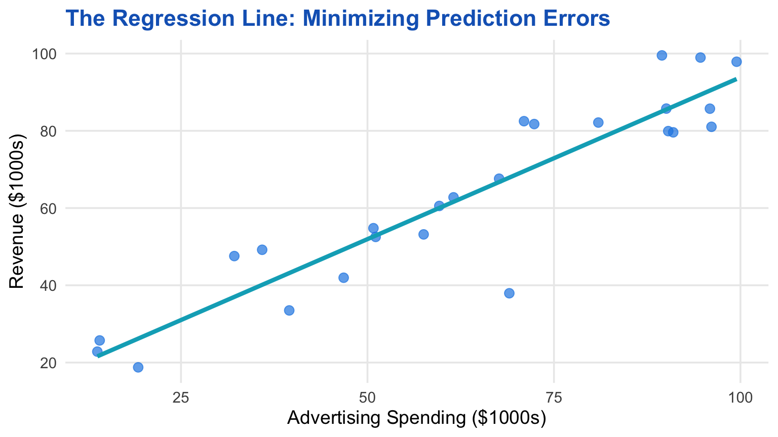
The Regression Line: “Line of Best Fit”

Goal: Find the line that minimizes the sum of squared errors (vertical distances from points to line)

This is called the Least Squares Regression Line

The Regression Equation

General Form

\[\widehat{y} = b_0 + b_1 x\]

Where:

$\widehat{y}$ (y-hat) = predicted value of y
$b_0$ = y-intercept (value of y when x = 0)
$b_1$ = slope (change in y for each 1-unit increase in x)
$x$ = value of the explanatory variable

For TechStart Ventures

\[\widehat{\text{Revenue}} = 12.45 + 0.78 \times \text{Advertising}\]

Intercept (12.45): Expected revenue with $0 advertising is $12,450
Slope (0.78): For each $1,000 increase in advertising, revenue is expected to increase by $780

Understanding the Slope

The slope ($b_1$) is the most important coefficient!

\[b_1 = r \times \frac{s_y}{s_x}\]

Where:

$r$ = correlation coefficient
$s_y$ = standard deviation of y
$s_x$ = standard deviation of x

Key Insight

The slope combines: 1. Correlation (how strong is the relationship?) 2. Relative variability (how much does y vary compared to x?)

For TechStart: $b_1 = 0.85 \times \frac{18.2}{19.7} = 0.78$

Making Predictions or Estimations

Example: A startup plans to spend $50,000 on advertising. What revenue do we predict?

Step 1: Identify the regression equation

\[\widehat{\text{Revenue}} = 12.45 + 0.78 \times \text{Advertising}\]

Step 2: Substitute x = 50

\[\widehat{\text{Revenue}} = 12.45 + 0.78 \times 50 = 12.45 + 39 = 51.45\]

Step 3: Interpret in context

We predict this startup will generate approximately $51,450 in revenue.

Warning

⚠️ Extrapolation warning: Only make predictions within the range of your data!

THINK-PAIR-SHARE 3 (7 minutes)

Using the TechStart regression equation:
$\widehat{\text{Revenue}} = 12.45 + 0.78 \times \text{Advertising}$

If advertising spending is $30,000, what revenue do we predict?

A. $24,850
B. $35,850
C. $42,450
D. $51,450

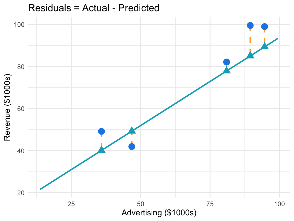
Residuals: Prediction Errors

Residual: The difference between actual and predicted values

\[e = y - \widehat{y}\]

Properties:

Positive: Actual > Predicted
Negative: Actual < Predicted
Sum of residuals = 0
Used to assess model fit

Good model: Small residuals

R-squared: “Goodness of Fit”

How much of the variability in y is explained by x?

\[R^2 = r^2\]

For TechStart Ventures

\[R^2 = (0.85)^2 = 0.72 = 72\%\]

Interpretation: 72% of the variability in Revenue is explained by Advertising spending.

Guidelines:

$R^2$ Value	Interpretation
0.00 - 0.30	Weak fit
0.30 - 0.70	Moderate fit
0.70 - 1.00	Strong fit

The remaining 28% is due to other factors (product quality, market timing, competition, etc.)

Google Sheets: Regression Analysis

Method 1: Using Functions

Slope: =SLOPE(known_y's, known_x's)
Intercept: =INTERCEPT(known_y's, known_x's)
R-squared: =RSQ(known_y's, known_x's)

Method 2: Built-in Regression Tool

Select your data (including headers)
Insert → Chart
Chart type: Scatter chart
Customize → Series → Trendline
Check “Show R²” and “Show equation”

data

Tip

The trendline method is fastest and visualizes everything at once!

THINK-PAIR-SHARE 4 (7 minutes)

A regression model has $R^2 = 0.40$.

What does this mean?

A. The correlation coefficient is 0.40
B. 40% of variability in y is explained by x
C. The model makes 40% errors
D. We’re 40% confident in predictions

Putting It All Together: TechStart Example

Complete Analysis

Research Question: Can we predict startup revenue from advertising spending?

Scatterplot: Shows clear positive linear relationship
Correlation: $r = 0.85$ (strong positive)
Regression Equation: $\widehat{\text{Revenue}} = 12.45 + 0.78 \times \text{Advertising}$
Interpretation:
- Each $1,000 in advertising predicts $780 increase in revenue
- With $0 advertising, predict $12,450 base revenue
Model Fit: $R^2 = 0.72$ (72% of revenue variability explained)
Prediction: For $50,000 advertising → predict $51,450 revenue

Key Concepts to Remember

Scatterplots visualize relationships between two quantitative variables
Correlation (r) measures strength and direction of linear relationships
- Range: -1 to +1
- Does NOT imply causation
Regression equation $\hat{y} = b_0 + b_1x$ models the relationship
- Intercept ($b_0$): Predicted y when x = 0
- Slope ($b_1$): Change in y per unit change in x
R-squared measures model fit (proportion of variability explained)
Use regression for prediction within data range (avoid extrapolation)

Looking Ahead: Next Lecture Preview

Next week: Inference with Regression

Is the relationship statistically significant?
Hypothesis tests for slope (is $b_1 \neq 0$?)
Confidence intervals for predictions
Standard error and prediction uncertainty
Conditions for regression inference

Coming Up

We’ll shift from describing relationships to making inferences about populations based on sample data!

Practice Problems

Try these before next class:

Calculate correlation for: Revenue vs Menu_price data (provided in the same shared Sheet)
Given: $\widehat{y} = -14.4 + 2.54x$
- Interpret the slope and intercept
- Predict y when x = 16
- If actual y = 40 when x = 10, what’s the residual?
If r = 0.95 and $R^2 = ?$ → What percentage of variability is explained?
Use Google Sheets to:
- Create a scatterplot
- Calculate correlation
- Add a trendline with equation

Questions? 💭

What questions do you have about:

Scatterplots?
Correlation?
Regression equations?
Making predictions?
Using Google Sheets?

Thank You! 🎉

See you next time for:

Inference with Regression

Office hours I’ll be here after class in case you need to talk

STAT 17: Linear Regression

📊 Case Study: TechStart Ventures

Learning Objectives 🎯

Why Linear Regression is Essential

📈 Descriptive Statistics

🔮 Inferential Statistics

Part 1: Visualizing Relationships 📉

Scatterplots

Scatterplots: The Foundation

THINK-PAIR-SHARE 1 (5 minutes)

Part 2: Quantifying Relationships 📏

The Correlation Coefficient

Correlation Coefficient (r)

Understanding Correlation Values

Google Sheets: Calculating Correlation

THINK-PAIR-SHARE 2 (7 minutes)

🍵 Break Time!

Part 3: Simple Linear Regression 📐

Building Prediction Equations

The Regression Line: “Line of Best Fit”

The Regression Equation

Understanding the Slope

Making Predictions or Estimations

THINK-PAIR-SHARE 3 (7 minutes)

Residuals: Prediction Errors

R-squared: “Goodness of Fit”

Google Sheets: Regression Analysis

THINK-PAIR-SHARE 4 (7 minutes)

Putting It All Together: TechStart Example

Key Concepts to Remember

Looking Ahead: Next Lecture Preview

Practice Problems

Questions? 💭

Thank You! 🎉