Mora_et_al2
Repository for code and data necessary to reproduce and replicate the paper: "First evidence for the aposematic function of a very common, but little-studied, color pattern in small insects."
- Experiments of spiders with live prey
- Experiment of spiders with false prey in automated cage
- Colophon
Experiments of spiders with live prey
Methods
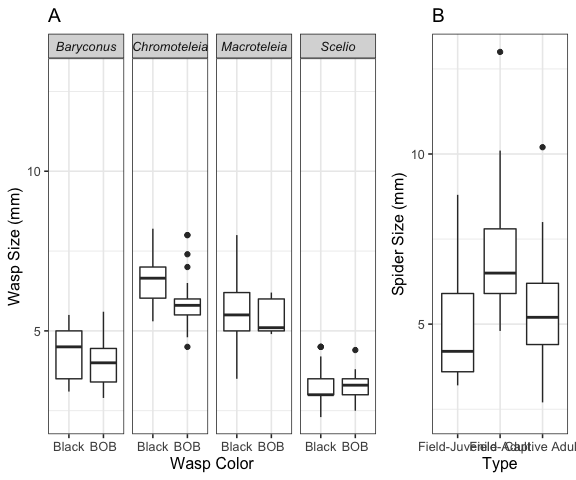
A total of 136 trials with three groups of spiders (68 field-juveniles, 51 field-adults and 17 captive-adults) and live prey were carried out during which the following data were recorded: spider type (juvenile, adult, reared), wasp color (BOB or black), spider behavior (behavioral scale explained before), time when the spider reacted (0-5, 5-10, 10-20, 20-30, 30-40 minutes), the distance between the spider and the prey during each behavior, presence/absence of a silk dragline, and wasp and spider body length. For each of the 136 trials consisting of a wasp with a spider, the size of each was measured (S3 Fig.). Although there is size variation within each group, predator (spiders) and prey (wasps) fall within the same general range, with field-captured adult spiders being the largest.
A multinomial logistic regression [26] was fitted to a simplified response: the most common activity for each spider was classified as “detect”, “attack” or “avoid”, in order to correct for zero or near zero counts in each response category. The full model includes the following covariates: wasp color, spider type, wasp size, spider size, wasp genus and presence/absence of silk dragline. This model was compared with simplified versions, with the result being that the model with wasp color and spider type was the model with the best fit, according to the AIC statistic. Additionally, frequency of actions for each group of spiders were calculated according to 10 minute slots, in order to define a clear timeline of spider behavior in the controlled experiments.
A separate experiment with lures in the automated cage included 30 trials, during which the following variables were recorded: presence/absence of silk dragline, spider size, background experimental arena color (black or white) and color of false prey (BOB vs black) that first attracted the spider. The response variable in this case was constructed by registering whether L. jemineus responded in the same way to black and BOB lures coded as 1, and whether L. jemineus responded in a different way to black and BOB lures coded as 2. Contingency tables were calculated, along with a Chi Square independence test for the response versus each of the variables: presence/absence of silk dragline, background color and prey color that first attracted the spider.
Results
For each of the 136 trials consisting of a wasp with a spider, the size of each was measured (Fig. 3 A, B). Although there is size variation within each group, predator (spiders) and prey (wasps) fall within the same general range, with field-captured adult spiders being the largest.
source(file="read_data.R")
## New names:
## * `` -> ...1
## * `` -> ...2
## * `Prey alert and swivel` -> `Prey alert and swivel...3`
## * `stalked and contact` -> `stalked and contact...4`
## * `detected and retrive` -> `detected and retrive...6`
## * ...
datos <- datos %>%
  mutate(s_type=recode_factor(s_type,
            "Field Juvenile"="Field-Juvenile",
            "Field Adult"="Field-Adult",
            "Captivity Adult"="Captive Adult"))
resumen <- datos %>% group_by(ID) %>%
  summarise(type=(unique(type)),
            typegr=(unique(typegr)),
            w_color=(unique(w_color)),
            w_size=(unique(w_size)),
            s_type=(unique(s_type)),
            s_size=(unique(s_size)),
            drag=(unique(drag))) %>% arrange(type, w_color, s_type)
## `summarise()` ungrouping output (override with `.groups` argument)
ftable(table(resumen$w_color,resumen$type))
##        Baryconus Chromoteleia Macroteleia Scelio
##
## Black          5           18          21     25
## BOB           15           37           5     10
ftable(table(resumen$w_color,resumen$typegr))
##        Baryconus Chrom. & Scelio Macroteleia
##
## Black          5              43          21
## BOB           15              47           5
ftable(table(resumen$w_color,resumen$s_type))
##        Field-Juvenile Field-Adult Captive Adult
##
## Black              25          36             8
## BOB                26          32             9
bp1 <- ggplot(resumen, aes(x=w_color, y=w_size)) +
  geom_boxplot()+ facet_wrap(~type, ncol=4)+theme(legend.position = "none")+
  # dejar la misma escala de spider size
  theme(strip.text = element_text(face = "italic"))+
  labs(title="A",x="Wasp Color", y = "Wasp Size (mm)") +
  ylim(c(min(resumen$w_size),max(resumen$s_size)))

bp2 <- ggplot(resumen, aes(x=s_type, y=s_size)) +
  geom_boxplot()+labs(title="B",x="Type", y = "Spider Size (mm)") +
  ylim(c(min(resumen$w_size),max(resumen$s_size)))

grid.arrange(bp1, bp2, nrow = 1, widths=2:1)
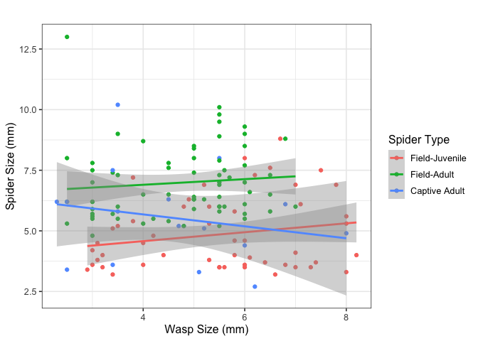
Association between sizes (not included in the paper):
bp <- ggplot(resumen, aes(x=w_size, y=s_size, color=s_type)) + geom_point()+ geom_smooth(method='lm', aes(color=s_type))+labs(color = "Spider Type")+
  labs(title="",x="Wasp Size (mm)", y = "Spider Size (mm)")
bp
## `geom_smooth()` using formula 'y ~ x'
summary(lm(s_size~w_size*s_type, data=resumen))
##
## Call:
## lm(formula = s_size ~ w_size * s_type, data = resumen)
##
## Residuals:
##     Min      1Q  Median      3Q     Max
## -2.6473 -1.1202 -0.3064  0.8690  6.2731
##
## Coefficients:
##                            Estimate Std. Error t value Pr(>|t|)
## (Intercept)                 3.84156    0.77749   4.941 2.35e-06 ***
## w_size                      0.18360    0.13588   1.351   0.1790
## s_typeField-Adult           2.59571    1.06576   2.436   0.0162 *
## s_typeCaptive Adult         2.82049    1.39012   2.029   0.0445 *
## w_size:s_typeField-Adult   -0.06774    0.20192  -0.335   0.7378
## w_size:s_typeCaptive Adult -0.42949    0.27400  -1.567   0.1194
## ---
## Signif. codes:  0 '***' 0.001 '**' 0.01 '*' 0.05 '.' 0.1 ' ' 1
##
## Residual standard error: 1.538 on 130 degrees of freedom
## Multiple R-squared:  0.3205, Adjusted R-squared:  0.2943
## F-statistic: 12.26 on 5 and 130 DF,  p-value: 9.581e-10
## Wrangle data:
datos <- datos %>%
  mutate(h_resp3=recode_factor(h_resp2,
                        "3.Crouch, jump and contact prey"="Attack",
                        "4.Pierce and ingestion"="Attack",
                        "1.Prey alert and swivel"="Detect",
                        "2.Follow or stalk"="Detect",
                        "5.Undetected or ignored"="Avoid",
                        "6.Detect visually and withdraw"="Avoid",
                        "7.None"="Avoid"))
d2<-datos %>% group_by(ID) %>% count(h_resp3) %>% top_n(1)
## Selecting by n
rep <- d2 %>% group_by(ID) %>% filter(n()>1) %>%
  summarize(h_resp3=unique(h_resp3)[1], n=n())
## `summarise()` ungrouping output (override with `.groups` argument)
datos2<-bind_rows(rep,d2[!d2$ID%in%rep$ID,]) %>% arrange(ID)
datos_model <- inner_join(datos2, resumen, by="ID")
with(datos_model, ftable(h_resp3,w_color, s_type))
##                 s_type Field-Juvenile Field-Adult Captive Adult
## h_resp3 w_color
## Attack  Black                       3           3             2
##         BOB                         4           0             2
## Detect  Black                      19          23             6
##         BOB                        18          28             5
## Avoid   Black                       3          10             0
##         BOB                         4           4             2
with(datos_model, ftable(h_resp3,w_color, type))
##                 type Baryconus Chromoteleia Macroteleia Scelio
## h_resp3 w_color
## Attack  Black                2            1           2      3
##         BOB                  5            0           0      1
## Detect  Black                3           13          15     17
##         BOB                  9           31           5      6
## Avoid   Black                0            4           4      5
##         BOB                  1            6           0      3
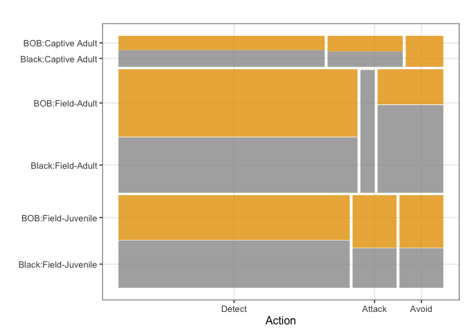
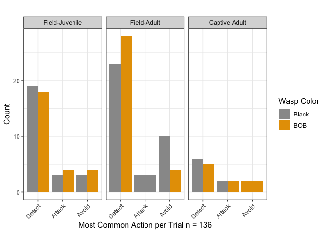
Multinomial Model
The multinomial logistic regression was fitted to a simplified response, where the most common activity for each spider was classified as “detect”, “attack” or “avoid”. A summary of the data included in the final model is presented in Figure 4. Note that in this figure the number of spiders differs between groups, which is why the bar for lab-reared (captive) adults is thinner than the ones for field adults and field juveniles. The full model includes the following covariates: wasp color, spider type, wasp size, spider size, wasp genus and presence/absence of silk dragline. This model was compared with simplified versions, with the result being that the model with presence/absence of silk dragline and spider type was the model with the best fit (AIC = 212.09).
datos_model$h_resp3 <- relevel(as.factor(datos_model$h_resp3),
                               ref = "Attack")
test00 <- multinom(h_resp3 ~ drag+s_type, data = datos_model)
test01 <- multinom(h_resp3 ~ s_type, data = datos_model)
test02 <- multinom(h_resp3 ~ s_type + w_color + type, data = datos_model)
test03 <- multinom(h_resp3 ~ s_type*w_color*type, data = datos_model)
test04 <- multinom(h_resp3 ~ s_type+w_color+s_size+w_size+drag+type, data = datos_model)
test05 <- multinom(h_resp3 ~ 1, data = datos_model)
c(test00$AIC,test01$AIC,test02$AIC,
  test03$AIC,test04$AIC,test05$AIC)
## [1] 212.0992 213.3870 213.4670 246.6749 220.1595 212.2821
test <- test00
summary(test)
## Call:
## multinom(formula = h_resp3 ~ drag + s_type, data = datos_model)
##
## Coefficients:
##        (Intercept)     drag s_typeField-Adult s_typeCaptive Adult
## Detect   -1.591937 1.824009          1.228139           -1.044539
## Avoid    -2.568090 1.459765          1.592933           -1.044696
##
## Std. Errors:
##        (Intercept)      drag s_typeField-Adult s_typeCaptive Adult
## Detect    1.365618 0.7574176         0.7471907           0.7584901
## Avoid     1.720320 0.9262931         0.8478523           1.0509646
##
## Residual Deviance: 196.0992
## AIC: 212.0992
z <- summary(test)$coefficients/summary(test)$standard.errors
p <- (1 - pnorm(abs(z), 0, 1)) * 2
p
##        (Intercept)       drag s_typeField-Adult s_typeCaptive Adult
## Detect   0.2437251 0.01603161        0.10024325           0.1684721
## Avoid    0.1354902 0.11504385        0.06027368           0.3202054
exp(summary(test)$coefficients)
##        (Intercept)     drag s_typeField-Adult s_typeCaptive Adult
## Detect  0.20353107 6.196653          3.414869           0.3518539
## Avoid   0.07668187 4.304950          4.918155           0.3517986
According to the aforementioned model, being a field adult is a significant factor for increasing the odds of detecting versus attacking (pvalue = 0.0108), and for avoiding versus attacking (pvalue = 0.0189). This shows that field adults are more likely to detect or avoid than to attack, compared to adults reared in captivity which appear to prefer attacking. Similarly, not using silk is associated with an increased chance of detecting versus attacking (pvalue = 0.0160), which makes sense since these spiders use silk only when attacking. Being a field-caught juvenile versus an adult reared in captivity did not make a difference in the most common spider actions. Other factors such as wasp color, wasp size, spider size, and wasp genus did not make a statistically significant difference when included in the full model. It should however be noted that field-caught adults only attacked black wasps, and adults reared in captivity avoided only BOB wasps.
datos_model <- datos_model %>%
  mutate(h_resp3=recode_factor(h_resp3, "Detect"="Detect","Attack"="Attack","Avoid"="Avoid"))
ggplot(data = datos_model) +
  geom_mosaic(aes(x = product(h_resp3, s_type),
              fill=w_color),
              show.legend=TRUE,
              na.rm=TRUE,
              divider=mosaic("v")) +
  theme(legend.position = "none") +
  scale_fill_manual(values=c("#999999", "#E69F00")) +
  labs(x = "Action", title='', y="")
# ggplot(data = datos_model) +
#   geom_mosaic(aes(x = product(h_resp3, s_type),
#               fill=w_color),
#               show.legend=TRUE,
#               na.rm=TRUE,
#               divider=mosaic("v")) +
#   theme(legend.position = "none") +
#   scale_fill_manual(values=c("#999999", "#E69F00")) +
#   labs(x = "Action", title='', y="")

ggplot(data=datos_model, aes(x=h_resp3, y=..count.., fill=w_color)) +
  geom_bar(position="dodge") +
  facet_wrap(~s_type, ncol=5)+
  scale_fill_manual(name = "Wasp Color", values=c("#999999", "#E69F00")) +
  labs(x = "Most Common Action per Trial n = 136", title='', y="Count")+
  #theme(legend.position = "none") +
  theme(axis.text.x = element_text(angle = 45, hjust = 1))
with(datos_model, ftable(h_resp3,w_color, s_type))
##                 s_type Field-Juvenile Field-Adult Captive Adult
## h_resp3 w_color
## Detect  Black                      19          23             6
##         BOB                        18          28             5
## Attack  Black                       3           3             2
##         BOB                         4           0             2
## Avoid   Black                       3          10             0
##         BOB                         4           4             2
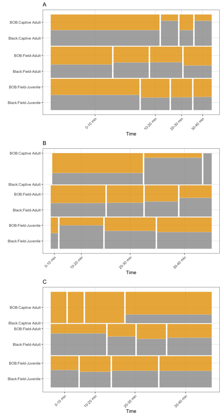
Timelines (original version)
options <- sort(unique(datos$h_resp3))
datos <- datos %>% mutate(time3= recode_factor(time2,
          "0-5 min"   = "0-10 min",
          "5-10 min"  = "0-10 min",
          "10-20 min" = "10-20 min",
          "20-30 min" = "20-30 min",
          "30-40 min" = "30-40 min"))
dat<-datos[datos$h_resp3=="Detect",]

ta1<- ggplot(data = dat) +
  geom_mosaic(data=dat,aes(x = product(w_color, time3),
                           fill=w_color,
                           conds=product(s_type)),
              na.rm=TRUE, divider=mosaic("v")) +
  scale_fill_manual(values=c("#999999", "#E69F00")) +
  labs(x = "Time", title='A', y="")+
  theme(legend.position = "none") +
  theme(axis.text.x = element_text(angle = 45, hjust = 1))

dat<-datos[datos$h_resp3=="Attack",]

ta2<- ggplot(data = dat) +
  geom_mosaic(data=dat,aes(x = product(w_color, time3),
                           fill=w_color,
                           conds=product(s_type)),
              na.rm=TRUE, divider=mosaic("v")) +
  scale_fill_manual(values=c("#999999", "#E69F00")) +
  labs(x = "Time", title='B', y="")+
  theme(legend.position = "none") +
  theme(axis.text.x = element_text(angle = 45, hjust = 1))

dat<-datos[datos$h_resp3=="Avoid",]

ta3<- ggplot(data = dat) +
  geom_mosaic(data=dat,aes(x = product(w_color, time3),
                           fill=w_color,
                           conds=product(s_type)),
              na.rm=TRUE, divider=mosaic("v")) +
  scale_fill_manual(values=c("#999999", "#E69F00")) +
  labs(x = "Time", title='C', y="")+
  theme(legend.position = "none") +
  theme(axis.text.x = element_text(angle = 45, hjust = 1))

grid.arrange(ta1, ta2, ta3, nrow = 3)
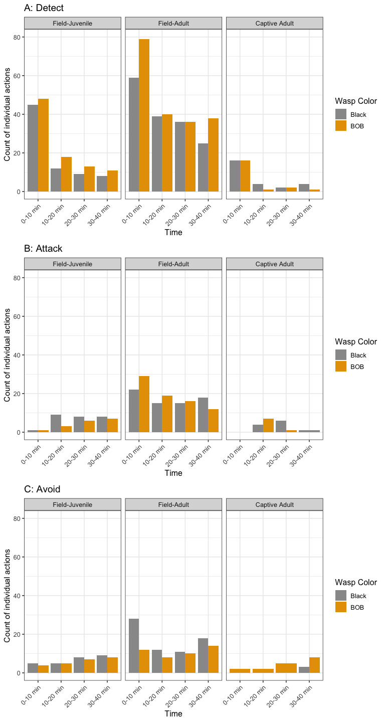
Timelines (bar plots option)
options <- sort(unique(datos$h_resp3))
dat<-datos[datos$h_resp3=="Detect",] %>%
  group_by(s_type, w_color, time3) %>% summarise(n=n())
## `summarise()` regrouping output by 's_type', 'w_color' (override with `.groups` argument)
t1<-   ggplot(data=dat, aes(x=time3, y=n, fill=w_color)) +
  geom_bar(stat="identity", position="dodge") + ylim(c(0,80))+
  facet_wrap(~s_type, ncol=5)+
  scale_fill_manual(name = "Wasp Color", values=c("#999999", "#E69F00")) +
  labs(x = "Time", title='A: Detect ', y="Count of individual actions")+
  #theme(legend.position = "none") +
  theme(axis.text.x = element_text(angle = 45, hjust = 1))

dat<-datos[datos$h_resp3=="Attack",]  %>%
  group_by(s_type, w_color, time3) %>% summarise(n=n())
## `summarise()` regrouping output by 's_type', 'w_color' (override with `.groups` argument)
t2<-  ggplot(data=dat, aes(x=time3, y=n, fill=w_color)) +
  geom_bar(stat="identity", position="dodge") + ylim(c(0,80))+
  facet_wrap(~s_type, ncol=5)+
  scale_fill_manual(name = "Wasp Color", values=c("#999999", "#E69F00")) +
  labs(x = "Time", title='B: Attack', y="Count of individual actions")+
  #theme(legend.position = "none") +
  theme(axis.text.x = element_text(angle = 45, hjust = 1))

dat<-datos[datos$h_resp3=="Avoid",]  %>%
  group_by(s_type, w_color, time3) %>% summarise(n=n())
## `summarise()` regrouping output by 's_type', 'w_color' (override with `.groups` argument)
t3<-   ggplot(data=dat, aes(x=time3, y=n, fill=w_color)) +
  geom_bar(stat="identity", position="dodge") + ylim(c(0,80))+
  facet_wrap(~s_type, ncol=5)+
  scale_fill_manual(name = "Wasp Color",values=c("#999999", "#E69F00")) +
  labs(x = "Time", title='C: Avoid', y="Count of individual actions")+
 # theme(legend.position = "none") +
  theme(axis.text.x = element_text(angle = 45, hjust = 1))

grid.arrange(t1, t2, t3, nrow = 3)
Re-coding of BOB for Table 1
# Re-code BOB and Black:
datos_model$w_color2<-if_else(datos_model$w_color=="Black","Black",
  if_else(datos_model$typegr =="Macroteleia"&datos_model$w_color=="BOB","BOB","PseudoBOB"))

datos_model <- datos_model %>%
  mutate(w_color2=recode_factor(w_color2, "Black"="Black",
                                "PseudoBOB"="PseudoBOB",
                                "BOB"="BOB"))

with(datos_model, ftable(type,w_color2,h_resp3))
##                        h_resp3 Detect Attack Avoid
## type         w_color2
## Baryconus    Black                  3      2     0
##              PseudoBOB              9      5     1
##              BOB                    0      0     0
## Chromoteleia Black                 13      1     4
##              PseudoBOB             31      0     6
##              BOB                    0      0     0
## Macroteleia  Black                 15      2     4
##              PseudoBOB              0      0     0
##              BOB                    5      0     0
## Scelio       Black                 17      3     5
##              PseudoBOB              6      1     3
##              BOB                    0      0     0
ftable(table(datos_model$w_color2,datos_model$h_resp3))
##            Detect Attack Avoid
##
## Black          48      8    13
## PseudoBOB      46      6    10
## BOB             5      0     0
ftable(table(datos_model$h_resp3,
             datos_model$s_type,
             datos_model$w_color))
##                        Black BOB
##
## Detect Field-Juvenile     19  18
##        Field-Adult        23  28
##        Captive Adult       6   5
## Attack Field-Juvenile      3   4
##        Field-Adult         3   0
##        Captive Adult       2   2
## Avoid  Field-Juvenile      3   4
##        Field-Adult        10   4
##        Captive Adult       0   2
datos_model <- datos_model %>%
  mutate(h_resp3=recode_factor(h_resp3, "Detect"="Detect",
                                "Attack"="Attack",
                                "Avoid"="Avoid"))
Experiment of spiders with false prey in automated cage
Methods
The experiment with false prey (lures) in the automated cage included 30 trials, during which the following variables were recorded: presence/absence of silk dragline, spider size, background experimental arena color (black or white) and color of false prey (BOB vs black) that first attracted the spider.
The response variable in this case was constructed following the algorithm:
- L. jemineus responded similarly to black and BOB lures = 1
- L. jemineus responded differently to black and BOB lures = 2
Contingency tables were calculated, along with a Chi Square independence test for the response versus each of the variables: presence/absence of silk dragline, background color and prey color that first attracted the spider.
Results
Table 1 presents the results from the experiment with false prey. Each contingency table was tested for independence, and the results were that there is no evidence of dependence in any of the cases. In other words, spider behaviors are not associated with background color, the color of lure that was detected first, the use or non-use of silk, or predator size.
library(DescTools)

names(datos_cont)
## [1] "n_exp" "backgr" "resp" "s_size" "silk" "first"
tab1<-table(datos_cont$resp,
            datos_cont$backgr)
GTest(tab1)
##
##  Log likelihood ratio (G-test) test of independence without correction
##
## data:  tab1
## G = 2.0879, X-squared df = 1, p-value = 0.1485
prop.table(tab1)
##
##                         Black     White
##   Different actions 0.2000000 0.1000000
##   Same actions      0.2666667 0.4333333
tab2<-table(datos_cont$resp,
            datos_cont$first)
GTest(tab2)
##
##  Log likelihood ratio (G-test) test of independence without correction
##
## data:  tab2
## G = 0.06728, X-squared df = 1, p-value = 0.7953
prop.table(tab2)
##
##                     Black BOB
##   Different actions   0.2 0.1
##   Same actions        0.5 0.2
tab3<-table(datos_cont$resp,
            datos_cont$silk)
GTest(tab3)
##
##  Log likelihood ratio (G-test) test of independence without correction
##
## data:  tab3
## G = 0.0089311, X-squared df = 1, p-value = 0.9247
prop.table(tab3)
##
##                        No silk       Silk
##   Different actions 0.23333333 0.06666667
##   Same actions      0.53333333 0.16666667
Statistical analysis was performed using the computing environment R (R Core Team, 2019). Data formatting and figures were prepared using the Tidyverse packages (Wickham, 2017). Multinomial logistic regression was done using the nnet package (Venables et al, 2002).
Colophon
This report was generated on 2020-12-02 20:47:35 using the following computational environment and dependencies:
# which R packages and versions?
if ("devtools" %in% installed.packages()) devtools::session_info()
## ─ Session info ───────────────────────────────────────────────────────────────
##  setting  value
##  version  R version 4.0.2 (2020-06-22)
##  os       macOS Catalina 10.15.7
##  system   x86_64, darwin17.0
##  ui       X11
##  language (EN)
##  collate  en_US.UTF-8
##  ctype    en_US.UTF-8
##  tz       America/Costa_Rica
##  date     2020-12-02
##
## ─ Packages ───────────────────────────────────────────────────────────────────
##  package      * version  date       lib source
##  assertthat     0.2.1    2019-03-21 [1] CRAN (R 4.0.2)
##  backports      1.1.10   2020-09-15 [1] CRAN (R 4.0.2)
##  blob           1.2.1    2020-01-20 [1] CRAN (R 4.0.2)
##  boot           1.3-25   2020-04-26 [1] CRAN (R 4.0.2)
##  broom          0.7.0    2020-07-09 [1] CRAN (R 4.0.2)
##  callr          3.5.1    2020-10-13 [1] CRAN (R 4.0.2)
##  cellranger     1.1.0    2016-07-27 [1] CRAN (R 4.0.2)
##  class          7.3-17   2020-04-26 [1] CRAN (R 4.0.2)
##  cli            2.2.0    2020-11-20 [1] CRAN (R 4.0.2)
##  colorspace     2.0-0    2020-11-11 [1] CRAN (R 4.0.2)
##  crayon         1.3.4    2017-09-16 [1] CRAN (R 4.0.2)
##  curl           4.3      2019-12-02 [1] CRAN (R 4.0.1)
##  data.table     1.13.2   2020-10-19 [1] CRAN (R 4.0.2)
##  DBI            1.1.0    2019-12-15 [1] CRAN (R 4.0.2)
##  dbplyr         1.4.4    2020-05-27 [1] CRAN (R 4.0.2)
##  desc           1.2.0    2018-05-01 [1] CRAN (R 4.0.2)
##  DescTools    * 0.99.38  2020-09-07 [1] CRAN (R 4.0.2)
##  devtools       2.3.2    2020-09-18 [1] CRAN (R 4.0.2)
##  digest         0.6.27   2020-10-24 [1] CRAN (R 4.0.2)
##  dplyr        * 1.0.2    2020-08-18 [1] CRAN (R 4.0.2)
##  e1071          1.7-3    2019-11-26 [1] CRAN (R 4.0.2)
##  ellipsis       0.3.1    2020-05-15 [1] CRAN (R 4.0.2)
##  evaluate       0.14     2019-05-28 [1] CRAN (R 4.0.1)
##  Exact          2.0      2019-10-14 [1] CRAN (R 4.0.2)
##  expm           0.999-5  2020-07-20 [1] CRAN (R 4.0.2)
##  extrafont    * 0.17     2014-12-08 [1] CRAN (R 4.0.2)
##  extrafontdb    1.0      2012-06-11 [1] CRAN (R 4.0.2)
##  fansi          0.4.1    2020-01-08 [1] CRAN (R 4.0.2)
##  farver         2.0.3    2020-01-16 [1] CRAN (R 4.0.2)
##  forcats      * 0.5.0    2020-03-01 [1] CRAN (R 4.0.2)
##  foreign      * 0.8-80   2020-05-24 [1] CRAN (R 4.0.2)
##  fs             1.5.0    2020-07-31 [1] CRAN (R 4.0.2)
##  generics       0.1.0    2020-10-31 [1] CRAN (R 4.0.2)
##  ggmosaic     * 0.3.1    2020-11-30 [1] Github (haleyjeppson/ggmosaic@c095f3a)
##  ggplot2      * 3.3.2    2020-06-19 [1] CRAN (R 4.0.2)
##  gld            2.6.2    2020-01-08 [1] CRAN (R 4.0.2)
##  glue           1.4.2    2020-08-27 [1] CRAN (R 4.0.2)
##  gridExtra    * 2.3      2017-09-09 [1] CRAN (R 4.0.2)
##  gtable         0.3.0    2019-03-25 [1] CRAN (R 4.0.2)
##  haven          2.3.1    2020-06-01 [1] CRAN (R 4.0.2)
##  hms            0.5.3    2020-01-08 [1] CRAN (R 4.0.2)
##  htmltools      0.5.0    2020-06-16 [1] CRAN (R 4.0.2)
##  htmlwidgets    1.5.2    2020-10-03 [1] CRAN (R 4.0.2)
##  httr           1.4.2    2020-07-20 [1] CRAN (R 4.0.2)
##  jsonlite       1.7.1    2020-09-07 [1] CRAN (R 4.0.2)
##  knitr          1.29     2020-06-23 [1] CRAN (R 4.0.2)
##  labeling       0.4.2    2020-10-20 [1] CRAN (R 4.0.2)
##  lattice        0.20-41  2020-04-02 [1] CRAN (R 4.0.2)
##  lazyeval       0.2.2    2019-03-15 [1] CRAN (R 4.0.2)
##  lifecycle      0.2.0    2020-03-06 [1] CRAN (R 4.0.2)
##  lmom           2.8      2019-03-12 [1] CRAN (R 4.0.2)
##  lubridate      1.7.9    2020-06-08 [1] CRAN (R 4.0.2)
##  magrittr       2.0.1    2020-11-17 [1] CRAN (R 4.0.2)
##  MASS           7.3-51.6 2020-04-26 [1] CRAN (R 4.0.2)
##  Matrix         1.2-18   2019-11-27 [1] CRAN (R 4.0.2)
##  memoise        1.1.0    2017-04-21 [1] CRAN (R 4.0.2)
##  mgcv           1.8-31   2019-11-09 [1] CRAN (R 4.0.2)
##  modelr         0.1.8    2020-05-19 [1] CRAN (R 4.0.2)
##  munsell        0.5.0    2018-06-12 [1] CRAN (R 4.0.2)
##  mvtnorm        1.1-1    2020-06-09 [1] CRAN (R 4.0.2)
##  nlme           3.1-148  2020-05-24 [1] CRAN (R 4.0.2)
##  nnet         * 7.3-14   2020-04-26 [1] CRAN (R 4.0.2)
##  pillar         1.4.7    2020-11-20 [1] CRAN (R 4.0.2)
##  pkgbuild       1.1.0    2020-07-13 [1] CRAN (R 4.0.2)
##  pkgconfig      2.0.3    2019-09-22 [1] CRAN (R 4.0.2)
##  pkgload        1.1.0    2020-05-29 [1] CRAN (R 4.0.2)
##  plotly         4.9.2.1  2020-04-04 [1] CRAN (R 4.0.2)
##  plyr           1.8.6    2020-03-03 [1] CRAN (R 4.0.2)
##  prettyunits    1.1.1    2020-01-24 [1] CRAN (R 4.0.2)
##  processx       3.4.5    2020-11-30 [1] CRAN (R 4.0.2)
##  productplots   0.1.1    2016-07-02 [1] CRAN (R 4.0.2)
##  ps             1.4.0    2020-10-07 [1] CRAN (R 4.0.2)
##  purrr        * 0.3.4    2020-04-17 [1] CRAN (R 4.0.2)
##  R6             2.5.0    2020-10-28 [1] CRAN (R 4.0.2)
##  Rcpp           1.0.5    2020-07-06 [1] CRAN (R 4.0.2)
##  readr        * 1.3.1    2018-12-21 [1] CRAN (R 4.0.2)
##  readxl       * 1.3.1    2019-03-13 [1] CRAN (R 4.0.2)
##  remotes        2.2.0    2020-07-21 [1] CRAN (R 4.0.2)
##  reprex         0.3.0    2019-05-16 [1] CRAN (R 4.0.2)
##  reshape2     * 1.4.4    2020-04-09 [1] CRAN (R 4.0.2)
##  rlang          0.4.9    2020-11-26 [1] CRAN (R 4.0.2)
##  rmarkdown      2.3      2020-06-18 [1] CRAN (R 4.0.2)
##  rprojroot      2.0.2    2020-11-15 [1] CRAN (R 4.0.2)
##  rstudioapi     0.13     2020-11-12 [1] CRAN (R 4.0.2)
##  Rttf2pt1       1.3.8    2020-01-10 [1] CRAN (R 4.0.2)
##  rvest          0.3.6    2020-07-25 [1] CRAN (R 4.0.2)
##  scales         1.1.1    2020-05-11 [1] CRAN (R 4.0.2)
##  sessioninfo    1.1.1    2018-11-05 [1] CRAN (R 4.0.2)
##  stringi        1.5.3    2020-09-09 [1] CRAN (R 4.0.2)
##  stringr      * 1.4.0    2019-02-10 [1] CRAN (R 4.0.2)
##  testthat       3.0.0    2020-10-31 [1] CRAN (R 4.0.2)
##  tibble       * 3.0.4    2020-10-12 [1] CRAN (R 4.0.2)
##  tidyr        * 1.1.2    2020-08-27 [1] CRAN (R 4.0.2)
##  tidyselect     1.1.0    2020-05-11 [1] CRAN (R 4.0.2)
##  tidyverse    * 1.3.0    2019-11-21 [1] CRAN (R 4.0.2)
##  usethis        1.6.3    2020-09-17 [1] CRAN (R 4.0.2)
##  vctrs          0.3.5    2020-11-17 [1] CRAN (R 4.0.2)
##  viridisLite    0.3.0    2018-02-01 [1] CRAN (R 4.0.1)
##  withr          2.3.0    2020-09-22 [1] CRAN (R 4.0.2)
##  xfun           0.17     2020-09-09 [1] CRAN (R 4.0.2)
##  xml2           1.3.2    2020-04-23 [1] CRAN (R 4.0.2)
##  yaml           2.2.1    2020-02-01 [1] CRAN (R 4.0.2)
##
## [1] /Library/Frameworks/R.framework/Versions/4.0/Resources/library
The current Git commit details are:
# what commit is this file at?
if ("git2r" %in% installed.packages() & git2r::in_repository(path = ".")) git2r::repository(here::here())
## Local:    master /Users/marce/Dropbox/Mora_CICIMA2
## Remote:   master @ origin (git@github.com:malfaro2/Mora_et_al2.git)
## Head:     [581de12] 2020-09-22: update plots mosaic