A study on Downscaling methods for Regional Climate Models

Marcela Alfaro Córdoba

Department of Statistics

This talk

Joint work with Luis Barboza, Shu Wei Chou, Hugo Hidalgo, and Eric Alfaro: Spatio-temporal downscaling emulator for regional climate models

• Motivation
• Methods and Model
• Simulation Studies
• Application to NARCCAP data
• Results and Findings

Epilogue: Lessons learned on reproducibility

Who am I?

• Assistant Professor of Teaching at the University of California SC

• Applied statistician - transition from a purely research career to a teaching focused career, but continuing with applied projects.

• My work on applied projects aims to develop a reproducible way to answer scientific questions with data. I use what I learn in this process to pass it on to my students when I design my courses.

Motivation

Downscaling

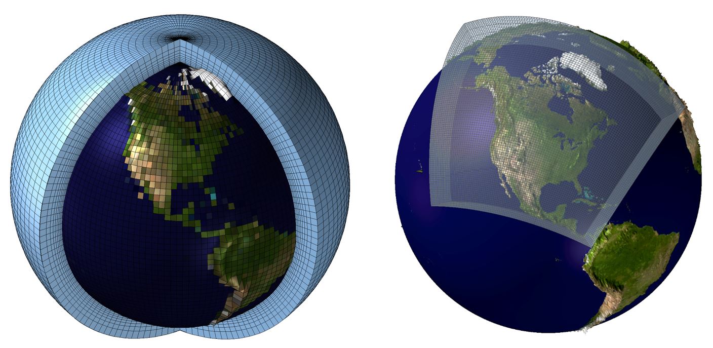
Downscaling is any procedure to infer high-resolution information from low-resolution variables. This technique is based on dynamical or statistical approaches.

Source: https://www.climatehubs.usda.gov/

Regional Climate Models (RCMs)

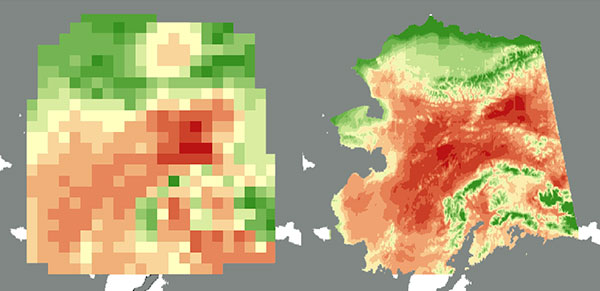
• RCMs use atmospheric and oceanic climate output in general circulation models (GCM) to develop a higher resolution climate output.

• They represent a tool for assessing climate variability and change impacts, to develop seasonal climate predictions, and are a powerful tool in general for improving our understanding of regional climate processes (Amador & Alfaro, 2009; Wang et al., 2004).

From Global Circulation Models (GCM) to Regional Climate Models (RCM)

Source: https://www.ouranos.ca/en/science-du-climat-modelisation-climatique

• RCMs are used to simulate climate variables at a regional scale. They are usually produced using dynamical downscaling, but they are computationally expensive and require high-performance computing resources.

From Global Circulation Models (GCM) to Regional Climate Models (RCM)

Source: https://www.ouranos.ca/en/science-du-climat-modelisation-climatique

• Using statistical downscaling methods, one can infer the values of RCMs from the output of global climate models (GCMs). This path is computationally cheaper and can be taken using personal computers.

NARCCAP Data

Source: https://narccap.ucar.edu/

• The North American Regional Climate Change Assessment Program (NARCCAP) is a multi-model experiment that provides high-resolution climate change scenarios for North America.

NARCCAP Data

Source: https://narccap.ucar.edu/

• One of the combinations included is the Community Climate System Model (CCSM) - a GCM - used to initialize the Canadian Regional Climate Model (CRCM).

How can we develop a statistical downscaling emulator that can use output from a GCM to infer the values of a regional climate model?

Objectives:

• Propose a statistical approach for downscaling climate variables from GCMs to RCMs, using a spatial varying coefficient model.
• Compare the performance of two estimation methods for said model.
• Show that it works properly using NARCCAP and observational data.
• Use the model with the output from the Community Climate System Model (CCSM - GCM) to infer the values of the Canadian Regional Climate Model (CRCM).

What has been done before?

• Statistical emulators: Castruccio et al. (2014), Overstall and Woods (2016), Mearns et al. (1999), O’Hagan (2006) and Hernanz et al. (2022) have been used on climate models’ projections and on computer experiment output.

• Spatio-temporal models as statistical emulators for storm surge models surge models (Hutchings et al., 2023), for modeling precipitation during tropical cyclones Kleiber et al. (2022) and to calibrate flood hazard models (Roth et al., 2022).

What has been done before?

• Other experiments to emulate regional models using downscaling techniques have been performed, as described in Wood et al. (2004) and Laflamme et al. (2016). However, they ignore the non-stationarity nature of the relationship between the GCM and RCM outputs.

• This is the first attempt to emulate RCM using varying coefficient models - the family of models presented by Gelfand et al. (2003). We aim to provide a quantification of uncertainty in the downscaling process, and to provide a model that can be used to predict the values of the RCM using the GCM output.

Model and Estimation

Model

\[\begin{align} C_t(s)=\alpha+\beta^\top X_t(s)+\epsilon_t(s), \label{eq-1} \end{align}\]

where:

• \(C_t(s)\): climate-related variable represented as a random variable \(C_t(s)\) indexed by time \(t\) and spatial location \(s\in S\).

• The spatial set \(S\) is assumed to be regularly-spaced with a fixed resolution.

• \(q\) covariates linearly related with the dependent variable \(C_t(s)\)

• \(\alpha\) and \(\beta\) are random parameters and \(\epsilon_t(s)\) is a white noise in both space and time with variance \(\zeta^2\).

Model

• Goal: Model the random field \(C_t(\cdot)\) over a set of finer resolution on the same spatial domain \(S\).
• We use \(W\) to be such set, and assume that the resolution satisfies that each location \(s\in S\) can be placed as a center of a rectangle containing several (or no) locations \(w_1,\ldots,w_K\) on the finer set \(W\).

Model

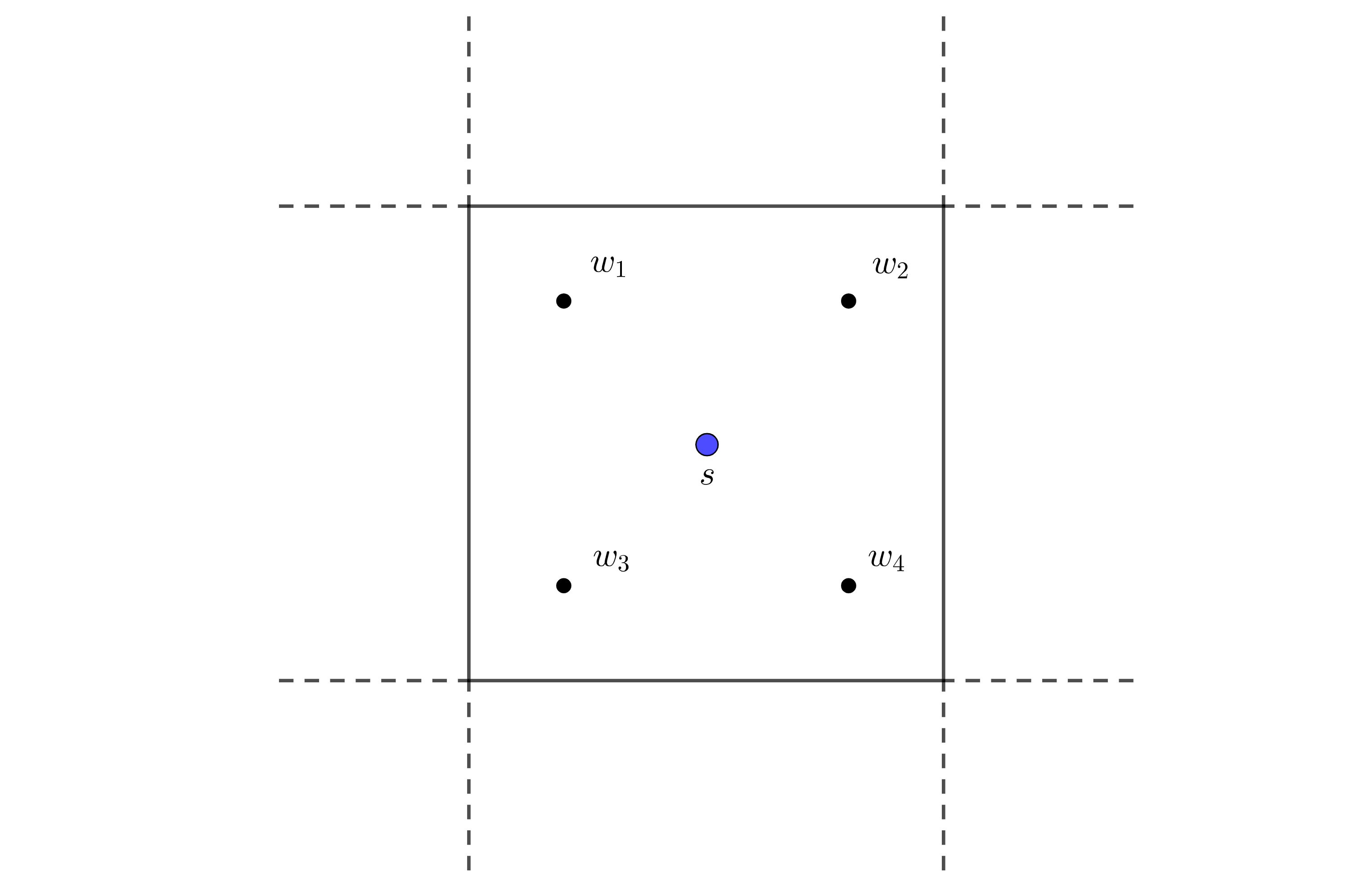
\[\begin{align} C_t(w)=[\alpha+\alpha_t^r(w)]+[\beta+\beta_t^r(w)]^\top X_t(s)+\epsilon_t(s)+\gamma_t(w), \end{align}\]

where

• \(\alpha_{\cdot}^r(\cdot)\sim N(\beta_0,\Sigma_0(\theta_0))\),
• \(\beta_{\cdot}^r(\cdot)\sim N(\beta_1,\Sigma_1(\theta_1))\),
• \(\gamma_t(\cdot)\stackrel{i.i.d}{\sim} N(0,\tau^2)\)
• \(\Sigma_0\) and \(\Sigma_1\) are separable spatio-temporal covariance matrices.

• Parameters \(\beta_0\) and \(\beta_1\) take into account any resulting bias due to the resolution change.
• The random terms \(\alpha_t^r(w)\), \(\beta_t^r(w)\) and \(\gamma_t(w)\) account for the increase in uncertainty due to the downscaling process.

Model

\[\begin{align} Y_t(w):=C_t(w)-C_t(s)=\alpha_t^r(w)+\beta_t^r(w)^\top X_t(s)+\gamma_t(w), \label{modelo} \end{align}\]

• \(C_t(s)\) is treated as a known covariate in this model and hence we are interested in the modeling of the difference \(Y_t(w)\) in order to get predictions on the finer variable \(C_t(w)\).

• \(\alpha_{\cdot}^r(\cdot)\) and \(\beta_{\cdot}^r(\cdot)\) represent random spatio-temporal correction terms on \(\alpha\) and \(\beta\) in the first equation due to the use of the predictor \(X_t(s)\) over the coarser set \(S\) and the change in scale between the sets \(S\) and \(W\).

Model

Under a Bayesian approach, we are interested in the conditional distribution of the dependent vector \(\mathbf Y:=(Y_t(w))_{t,w}\) given the parameters \(\Phi:=(\beta_0,\beta_1,\theta_0,\theta_1, \tau^2)\): \[\begin{align*} \mathbf Y|\Phi \sim N(\beta_0+\mathbf X^\top \beta_1,\Sigma_Y), \end{align*}\] where \[\begin{align*} \Sigma_{\mathbf Y}=\mathbf X^\top \left(\Sigma_0(\theta_0)+\Sigma_1(\theta_1)\right) \mathbf X+\tau^2 I_n \end{align*}\] and \(\mathbf X\) is a block-diagonal matrix whose \(i\)-th sub-matrix is \(X^\top(s_i)\), \(i=1,\ldots,n\) and \(n\) is the number of locations in \(S\).

Estimation

• In order to evaluate the likelihood of \(\mathbf Y\) we need to evaluate the inverse and determinant of \(\Sigma_{\mathbf Y}\) which can be time-consuming for a combination of a large \(n\) and/or a large number of times \(t\).

• We compare two estimation methods:

  • Integrated Nested Laplace Approximation (INLA)

  • The approach developed by Dambon et al. (2021) using the varycoef R package and adapting it to a Bayesian framework.

Estimation - INLA

The INLA approach is applicable to a general specification for which the mean \(\eta_i\) of the observations \(y_i\) follows a linear structure: \[\begin{align}\label{eq:meanINLA} \eta_i = \alpha +\sum_{m=1}^M\beta_mx_{mi}+\sum_{l=1}^Lf_l(z_{li}), \end{align}\] where \(\alpha\) represents an intercept, the coefficients \(\mathbf{\beta} = (\beta_1,\ldots,\beta_M)\) relate \(M\) covariates \((x_1,\ldots,x_M)\) to \(\eta_i\), and \(f = \{f_1(\cdot),\ldots,f_L(\cdot)\}\) is a collection of random effects defined on a set of \(L\) covariates \((z_1,\ldots,z_L)\) (Rue 2009 and Blangiardo 2013).

Estimation - INLA

• Let \(y_i=\eta_i=Y_t(w)\) and the varying intercept and slope are the latent variables with fixed effects as their respective means \(\beta_0\) and \(\beta_1\), then our models fall into the general specification of INLA.

• INLA assumes that the prior of vector \(\Phi\) is a multivariate normal random vector with a precision matrix that depends on a certain set of hyperparameters.

• INLA further approximates the conditional distribution of \(\Phi\) by using a simplified Laplace Approximation together with optimization procedures (Rue 2009).

Estimation - Dambon et al. (2021)

This approach has two important assumptions:

• Mutual prior independence of the random effects \(\alpha^r(\cdot)\) and \(\beta^r(\cdot)\),
• Each random effect has tapering on its covariance matrix.

\[\begin{align} \Sigma_Y=\sum_{i=1}^p \Sigma^{j} \odot \mathbf X^{j}+\tau^2 I_n, \end{align}\]

where \(\odot\) is the Hadamard product and \(\mathbf X^{j}:= x^{(j)}\left(x^{(j)}\right)^\top\) uses the \(j\)th covariate \(x^{(j)}\).

Estimation - Dambon et al. (2021)

The covariance matrix can be simplified as:

\[\begin{align} \Sigma_{Y,tap}=\sum_{i=1}^p \Sigma_{tap}^{j} \odot \mathbf X^{j}+\tau^2 I_n. \end{align}\]

The tapering, together with the sparsity of the matrix \(\textbf{X}\) reduces the execution time. This approach is fully implemented with maximum likelihood estimation using the R package varycoef, available on CRAN. We adapted the approach by using MCMC estimation.

Simulation Studies

Simulation Studies

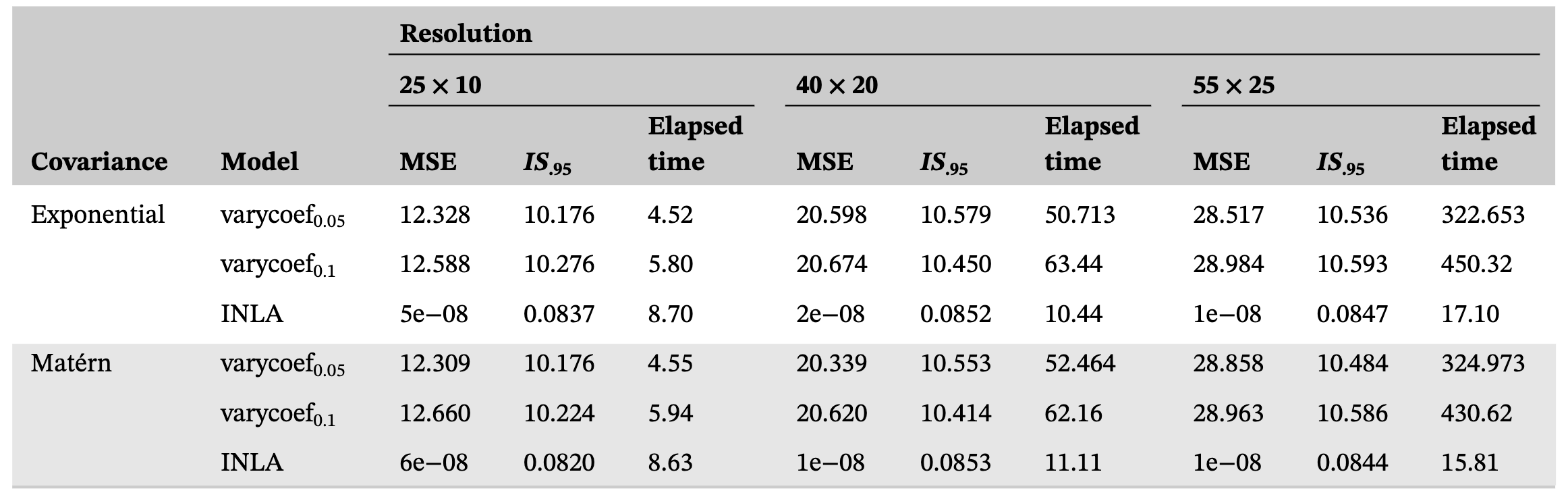
First. Comparing the performance of the INLA and Dambon et al. (2021) approaches in terms of predictive capacity and computational time.

Second study. Evaluating the performance of the proposed emulator in terms of predictive capacity and computational time, using the best estimation method from the first study.

Simulation Studies

Statistics used to evaluate the performance of the emulator:

• Mean Squared Error (MSE)
• Elapsed Time (in minutes)
• Interval Score (Gneiting, 2007): an utility function in interval estimation that addresses width as well as coverage. It is defined as:

\[\begin{align} \mathit{IS}_{\alpha}=\frac 1 n \sum_{t,w}\left[(U_t(w)-L_t(w))+\frac{2}{1-\alpha}(L_t(w)-Y_t(w))\cdot 1_{Y_t(w)<L_t(w)}\right. \\ \left.+\frac{2}{1-\alpha}(Y_t(w)-U_t(w))\cdot 1_{Y_t(w)>U_t(w)}\right], \end{align}\]

Simulation Study - First

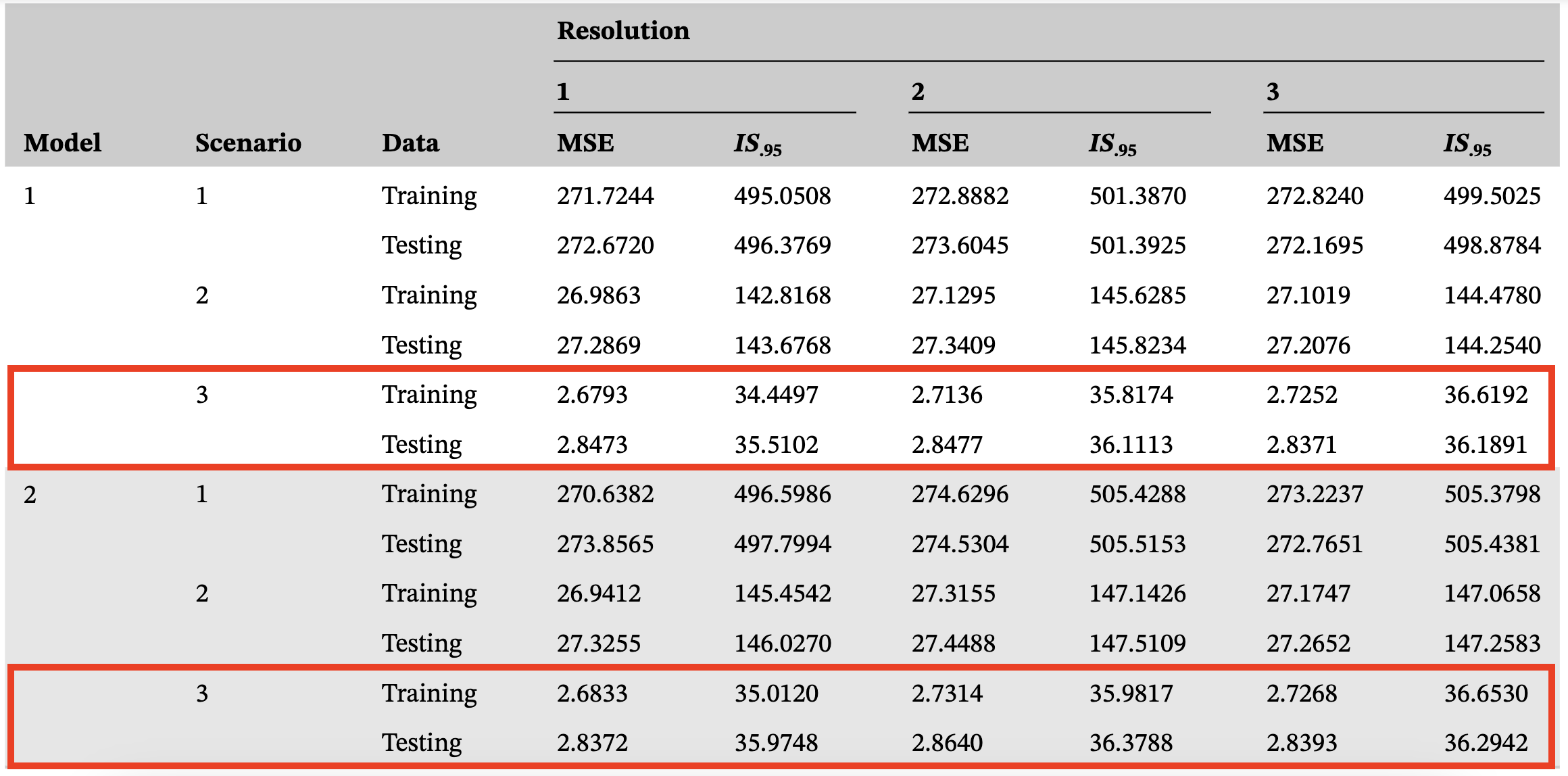
• In the spatial region \(\left[0,1\right]^2\), we set three different resolutions for the regularly-spaced set \(S\) and the finer set \(W\). We use \(25 \times 10\), \(40 \times 20\) and \(55 \times 25\) as three different resolution scenarios for this simulation and for each scenario we generate 10 replications.

• At these locations, we simulate two models fixing \(q=1\), \(\alpha=5.6\), \(\beta_0=-0.05\), \(\beta=0.015\), \(\beta_1=-0.005\), \(\zeta^2=2\) and \(\tau^2=1\).

• We consider a spatially varying intercept with a spatial covariance structure following either a Matérn \((\phi=0.1,\sigma=0.001,\nu=0.8)\) or an Exponential\((\phi=0.1,\sigma=0.001)\).

Simulation Study - First

Simulation Studies - Second

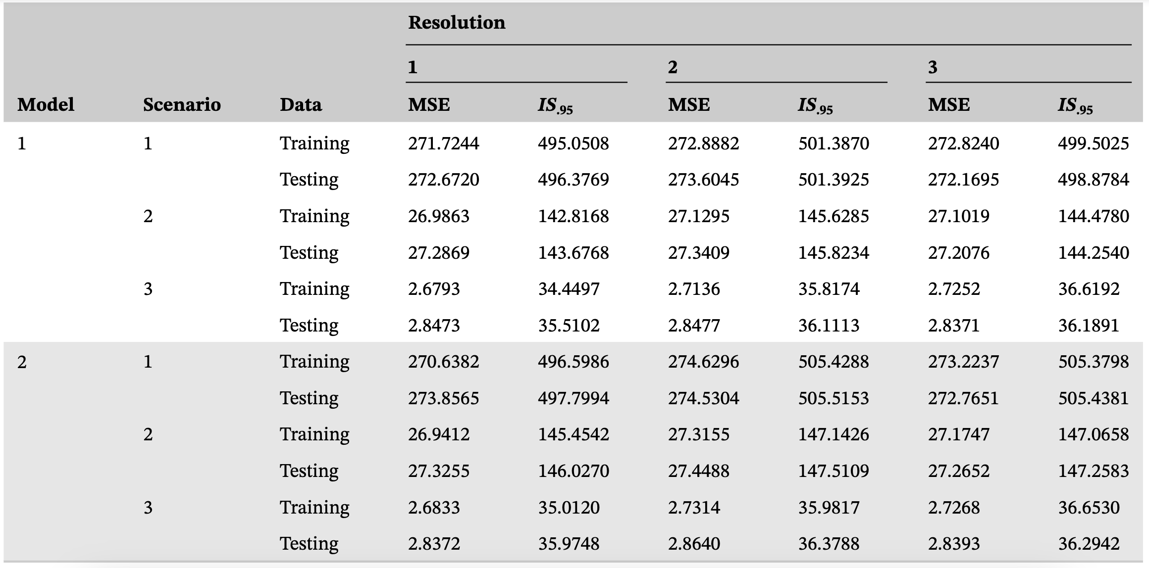
• In the spatial region \(\left[0,20\right]^2\), we set three different resolutions for the regularly-spaced set \(S\) and the finer set \(W\). We use \((20 \times 10)\) as Resolution 1, \((40 \times 20)\) as Resolution 2, and \((60 \times 10)\) as Resolution 3.

• \(T=12\) periods of time were simulated for each scenario. For each simulated data, we divided it into two sets: a training data set containing the first \(5/6\) periods of time, and a testing data set, containing the last \(1/6\) periods of time.

Simulation Studies - Second

• For the three different variability scenarios, we set the spatial varying intercept \(\alpha_r(\omega)\) with spatial covariance structure Matérn \(\theta_0\) with \(\theta_0=(\phi=5,\sigma ,\nu=1)\), where \(\sigma= 0.003,0.0003,0.00003\). Recall that \(\phi\) and \(\sigma\) are known as the range and variance parameters of the Matérn covariance structure and \(\nu\) is its smoothness parameter. For each of the nine scenarios we generate 30 replications.

Simulation Studies - Second

Simulation Studies - Second

Simulation Studies - Results

• The INLA method outperformed the Dambon approach in terms of predictive capacity and computational time for fitting the proposed emulator model.

• The emulator showed potential for accurately predicting RCM output using GCM output, with good out-of-sample predictive performance.

• The elapsed time for the emulator was around 1 min for all scenarios, which is a reasonable time for a model with a large number of parameters.

Application to NARCCAP data

Data

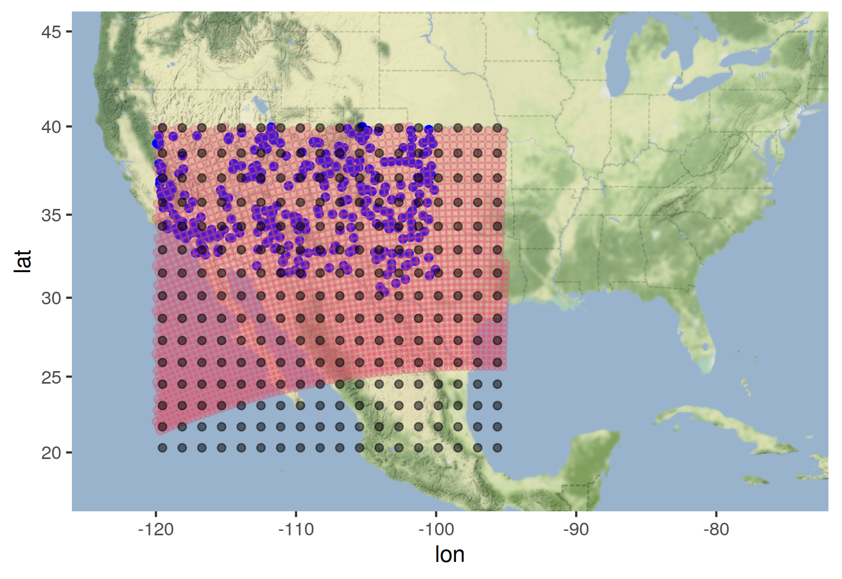
Coordinates for the Canadian Regional Climate Model (CRCM) (red points), the Community Climate System Model (CCSM) in the North American Region (black points) and observed temperatures (blue points).

Data

• Mean air surface temperature (ts) measured in Kelvin from the Canadian Regional Climate Model (CRCM) (Caya et al., 1995),

• Seasonal mean pressure vertical velocity measured in Pa/s (OMEGA) and mean air surface temperature (TREFHT) measured in Kelvin from Community Climate System Model (CCSM) (Mearns et al., 2007).

• 2482 points in the regional-model resolution grid, and 270 points for the global-based one. Monthly data from 1990 to 1998 (inclusive) was used to fit the model

• 180 observed surface air temperature records from the National Climatic Data Center (NCDC) (Groisman et al. (2004) and Alfaro et al. (2006)) to test the results.

Models

• The main objective of the emulator is to use the CCSM output to infer the values of the CRCM output.

• There is a non-stationary relationship between the CCSM output and the regional model response.

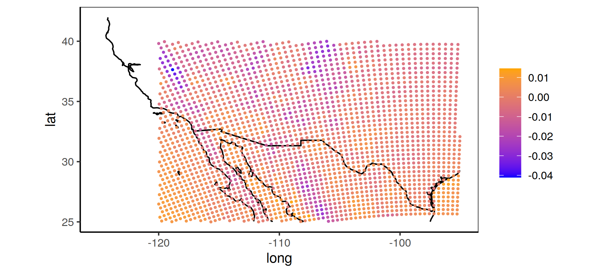
Mean difference between the monthly temperature log-outputs among the regional and global models (1990-1999)

Models

\[\begin{align} Y_t(w):=C_t(w)-C_t(s)=\alpha_t^r(w)+\beta_t^r(w)^\top X_t(s)+\gamma_t(w), \end{align}\]

• \(C_t(\cdot) = \log T_t(\cdot)\), where \(T_t\) is the temperature and the domains \(S\) and \(W\) correspond to the global and regional domains respectively.
• \(X_t(\cdot) = OMEGA_t(\cdot)\) Vertical rising rate of air parcels. Provides a measure of large scale rising and sinking motions in the atmosphere. It was obtained from the CCSM model.

Models

• Model 0: Non varying intercept model.
• Model 1: Spatio-temporal varying intercept following a random noise process, where the spatial covariance structure follows a Matérn\(\left(\nu=1 \right)\).
• Model 2: Spatio-temporal varying intercept following an \(AR(1)\) process, where the spatial covariance structure follows a Matérn\((\nu= 1)\).
• Model 3: Spatio-temporal varying intercept following an \(AR(1)\) process with a fixed-parameter covariate.

Results

Results

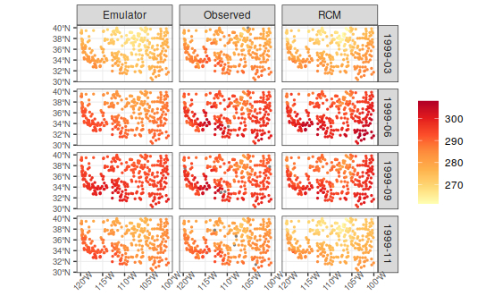
Estimated temperatures according to Model 1 (emulator), observed temperatures and RCM.

Results

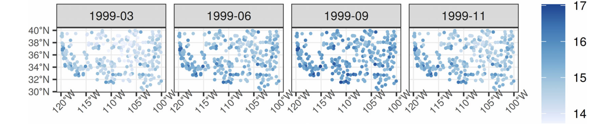
Interquartile range for four chosen months during the testing period. Missing values are drawn in gray.

Conclusions and findings

Conclusions and findings

• A spatio-temporal downscaling emulator for regional models was proposed using spatial varying coefficients. The model can estimate non-stationary marginal effects, which means that the downscaling function can vary over space.

• INLA was the best method to estimate the spatial and spatial temporal versions of the proposed model, when compared with the Dambon et al. (2021) approach, under different tapering coefficients.

• The model has good prediction results for reproducing the annual cycles for one particular year, as shown on both the simulation results, and the analysis of NARCCAP data. These good results in terms of prediction happens in spite of the possible identification issues observed in the same sections.

Conclusions and findings

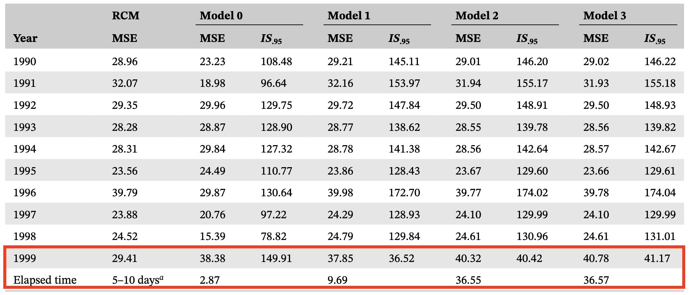
• The downscaling emulator showed potential for predicting accurately output from RCM using the output from a GCM. Specifically, temperature from the CRCM can be predicted using mean pressure vertical velocity output from CCSM with an out of sample MSE of approximately 34 units for all models proposed, and with a \(95\%\) IS that is significantly lower for Models 2 and 3, compared to the other options.

• Furthermore, when adding the elapsed time to run the models, and given that Model 1 and Model 2 give very similar predictive performance results, then Model 1 is preferred, since it can be run in less than one third of the time that takes to complete Model 2.

Computational Resources

• HP Proliant DL380 Gen9 server, Intel(R) Xeon(R) CPU E5-2630 v3 @ 2.40GHz, with16 logical cores, and 128GB RAM.

• The R scripts to read and wrangle the NARCCAP data, as well to run all of the models described in this article are available at https://github.com/LEA-UCR/MRA-ST and were run using RStudio Server2022.02.2 Build 485. Packages and R version are specified in the Readme repository file.

Epilogue

Lessons on Reproducibility

• The importance of reproducibility in scientific research is well known, but it is not always easy to achieve.

• JASA Reproducible Research Recommendations (2017)

  • Data and code availability
  • Documentation
  • Use of open source software
  • Version control
  • Reproducible workflow
  • Reproducible environment

Lessons on Reproducibility

• Reproducibility is not a binary state. We can take small steps to improve the reproducibility of our work.
• The best way to learn about reproducibility is to practice it.
• It takes time and resources to be reproducible, but it is worth it. And hopefully, it will be absolutely necessary in the future.
• One part of reproducibility often neglected is the documentation of the code to scrap, read, format and preprocess your data.
• Using version control when collaborating in a team is essential. However, this requires that all team members are familiar with the tool you are using.

Lessons on Reproducibility

• An excellent way to promote reproducibility is to incorporate it in our classrooms.
  • Assignments that require reproducible reports
  • Use of version control in group projects
  • Use of Quarto and/or Rmarkdown for lab reports
  • Use of open source software in the classroom
  • Use of LLMs to document code
  • ReproHacks and ReproSprints
  • Reproducibility workshops

Thank you!

Questions?

References

References 1

Article (with references): https://onlinelibrary.wiley.com/doi/epdf/10.1002/env.2815

Data: https://www.narccap.ucar.edu/data/

Code: https://github.com/LEA-UCR/MRA-ST

References 2

Reproducible analysis references:

• Alston et al (2021) A Beginner’s Guide to Conducting Reproducible Research https://esajournals.onlinelibrary.wiley.com/doi/full/10.1002/bes2.1801

• Broman et al (2017) Recommendations to Funding Agencies for Supporting Reproducible Research https://www.amstat.org/asa/files/pdfs/POL-ReproducibleResearchRecommendations.pdf

• JASA Reproducibility Guide https://jasa-acs.github.io/repro-guide/pages/acc.html