Linear Regression in Practice

Week 5 · Tuesday, Oct 27 · Lecture + AI audit #1

Dr. Marcela Alfaro Córdoba

Today’s plan

Time	What
1:30	DS 5 check: swap laptops
1:45	Fitting a line: `lm()`, slope, intercept, prediction
2:10	How good is the line? `summary()` and residuals
2:25	AI audit #1, in groups
2:55	Your project’s first model

Learning goals: fit and plot a one-predictor linear model, read its slope, R² and p-value in the units of the data, and check the residuals before believing any of it.

DS 5 check

Swap laptops

⏱ 10 min

Swap laptops with your neighbor. On their laptop, open week05/ds05_notes.R:

Restart test: Session → Restart R, then source the script. Does it run with no errors?
Break a function: call their knots_to_kmh() with "fast" and with -3. Does it stop, with a clear message?
Compare one exercise with yours. Different numbers are expected. Is the code doing the same thing?
Read their two comments at the bottom. Can you help with either one?

At the top of their script, add: # Checked by <your name>: one thing that works, one question

Then, back on your own laptop

On the Ed thread “DS 5 check”, post two lines:

The hardest part to understand this week
Something that hasn’t quite clicked yet

Note

This is today’s 1-point discussion check: a careful swap, a comment left in your classmate’s script, and your Ed post. I read every post, and they decide what we review next week.

Fitting a line

A question worth a line

Do people in richer countries live longer? One year, 142 countries:

library(ggplot2)
gm07 <- gapminder[gapminder$year == 2007, ]
ggplot(gm07, aes(x = gdpPercap, y = lifeExp)) +
  geom_point() +
  scale_x_log10() +
  geom_smooth(method = "lm", se = FALSE)

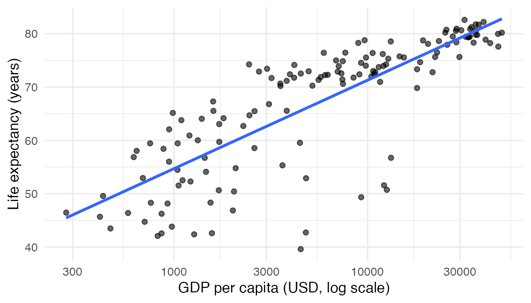
Week 4’s plot. Today: the numbers behind that blue line.

`lm()`: a linear model

fit <- lm(lifeExp ~ log10(gdpPercap), data = gm07)
fit
#> Coefficients:
#>      (Intercept)  log10(gdpPercap)
#>             4.95             16.59

Piece	Means
`lifeExp ~ log10(gdpPercap)`	“life expectancy explained by log GDP”: response on the left of `~`
`data = gm07`	where to find those columns
`fit`	a model object: estimates, fitted values, residuals, all inside

Why log10()? Week 4: on a log scale the cloud is a straight line. On the raw scale it isn’t, and a straight line won’t fit it. Hold that thought until the audit.

Read the slope in the units of the data

coef(fit)
#>      (Intercept) log10(gdpPercap)
#>         4.949612        16.585064

Slope, 16.6: one step on log10(gdpPercap) is a ten-fold increase in GDP per capita. So:

Countries with ten times the income have, on average, a predicted life expectancy 16.6 years higher.

Intercept, 4.95: the prediction when log10(gdpPercap) is 0, at $1 per person. No country is near that (the poorest is about $278). It positions the line; it means nothing on its own.

Predictions

a <- coef(fit)[1]
b <- coef(fit)[2]
a + b * log10(5000)                                      #> 66.29726

predict(fit, newdata = data.frame(gdpPercap = 5000))     #> 66.29726

predict() does the arithmetic, and applies the log10() for you
newdata must have a column with the same name as the predictor in the formula

Warning

Predict only inside the range of your data: here, about $278 to $49,357. Outside it, the line is a guess with decimals.

Your turn: two predictions

⏱ 5 min

In a new script, week05/regression.R:

Fit fit, as above
Predict life expectancy at $1,000 and at $10,000, with one call to predict()
Subtract the two predictions. Where have you seen that number before?

p <- predict(fit, newdata = data.frame(gdpPercap = c(1000, 10000)))
p          #>        1        2
           #> 54.70480 71.28987
diff(p)    #> 16.58506

$1,000 to $10,000 is a ten-fold increase, so the difference is the slope. predict() is vectorized, like everything on Thursday.

How good is the line?

`summary()`: read three numbers

summary(fit)
#> Coefficients:
#>                  Estimate Std. Error t value Pr(>|t|)
#> (Intercept)         4.950      3.858   1.283    0.202
#> log10(gdpPercap)   16.585      1.019  16.283   <2e-16 ***
#> ...
#> Multiple R-squared:  0.6544, Adjusted R-squared:  0.652

Number	Here	What it says
Estimate	16.585	the slope, same as `coef()`
`Pr(>\|t\|)` for the slope	< 2e-16	a slope this far from 0 would be very unlikely if there were no linear relationship
R²	0.654	the line accounts for 65% of the variation in life expectancy

A small p-value says the slope isn’t zero. It says nothing about how big, how important, or how causal the relationship is.

Residuals: what the line misses

gm07$resid <- residuals(fit)       # observed minus predicted
head(gm07[order(gm07$resid), c("country", "lifeExp", "gdpPercap", "resid")], 4)
#>           country lifeExp gdpPercap     resid
#> 1464    Swaziland  39.613  4513.481 -25.94692
#> 48         Angola  42.731  4797.231 -23.26808
#> 168      Botswana  50.728 12569.852 -22.20926
#> 1416 South Africa  49.339  9269.658 -21.40462

Swaziland (now Eswatini) lives about 26 years shorter than its income predicts. Southern Africa in 2007 was at the height of the HIV/AIDS epidemic. The biggest residuals are often the most interesting part of an analysis.

The residual plot

ggplot(gm07, aes(x = fitted(fit), y = resid)) +
  geom_point() +
  geom_hline(yintercept = 0)

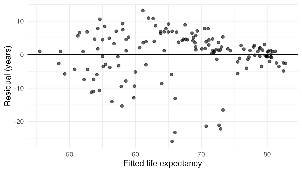
What you hope for: a shapeless cloud around 0. A curve means the straight line is missing something; a funnel means the spread changes. Here: mostly a cloud, with a long tail of countries far below the line.

Check how many rows the model used

The survey: do people who live farther away visit the library less?

fit_s <- lm(visits ~ commute_min, data = survey)
coef(fit_s)       #>  (Intercept)  commute_min
                  #>  3.533586707 -0.001677429
nobs(fit_s)       #> [1] 44

44, not 45: lm() quietly dropped the row with a missing commute (id 35). You knew about it from Week 3. Did you know lm() would drop it?
Slope ≈ 0, R² ≈ 0, p = 0.96: no linear relationship in these data. That’s a result too

Tip

After every lm(): nobs(fit). If the number surprises you, go back to your cleaning script.

A line is not a cause

“Associated with”, not “causes”, “increases” or “leads to”.

Income, health systems, education, history and conflict are all tangled together
The model can’t tell you that raising a country’s GDP will raise its life expectancy
It describes these data: 142 countries, 2007

This is the sentence AI tools get wrong most often. Which brings us to the audit.

AI audit #1

The task

⏱ 15 min

In groups of 3. The next slide is a regression analysis written by an AI, for the same question and data we just used. It runs without errors.

Find everything that is wrong or misleading. There are at least five problems
For each: what’s wrong, how you found it, and the corrected sentence or code
Run the code if it helps. You may not ask another AI

Then 10 minutes together. Each group reports one problem, and how they found it. The “how” is the skill.

The AI’s analysis

gm07 <- gapminder[gapminder$year == 2007, ]
fit <- lm(lifeExp ~ gdpPercap, data = gm07)
summary(fit)       # slope 0.000637, intercept 59.57, R² 0.461, p < 2e-16
predict(fit, newdata = data.frame(gdpPercap = 100000))     #> 123.2791

Results. GDP per capita has a highly significant positive effect on life expectancy (p < 0.001). The intercept shows that the average life expectancy in 2007 was 59.6 years. Each additional $10,000 of GDP per capita increases life expectancy by 6.4 years. The model is 46% accurate (R² = 0.46). A country with a GDP per capita of $100,000 would have a life expectancy of 123 years.

Conclusion. Because the p-value is so small, GDP is the most important factor determining life expectancy. Countries should prioritize economic growth to improve health.

What we found: the numbers

AI says	Problem	How you’d find it
(no plot) a straight line on raw GDP	Unchecked assumption. The relationship is curved	Plot it; residual plot shows a clear curve. With `log10()`: R² 0.65 vs 0.46
“average life expectancy was 59.6”	Misread intercept. It’s the prediction at $0 \| `mean(gm07$lifeExp)`is 67.0 \| \| "46% accurate" \| Misread R². It's the share of variation explained \| Lesson 11, or`?summary.lm`

What we found: the conclusions

AI says	Problem	How you’d find it
“$100,000 → 123 years”	Extrapolation. The data stop at $49,357 \| `range(gm07$gdpPercap)`; nobody lives 123 years
“increases”, “should prioritize growth”	Causal claim from observational data	Ask: what else differs between rich and poor countries?
“most important factor”	p-value misread as importance	A p-value is not a size; there’s only one predictor to compare

The plot the AI never made

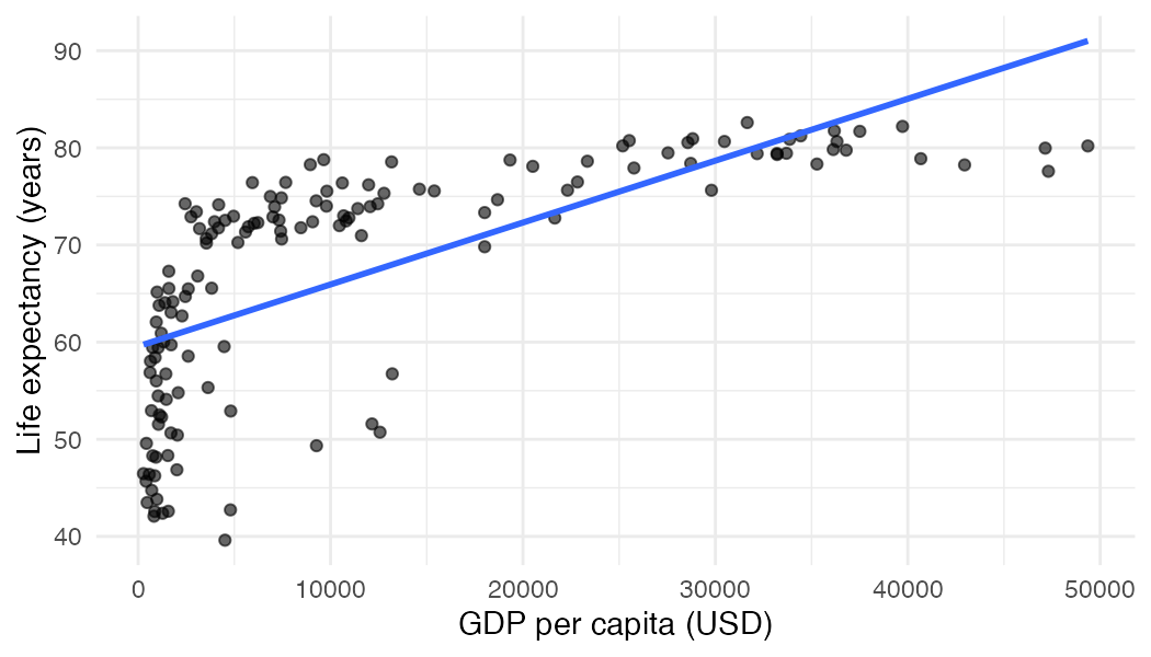
The straight line on the raw scale: too high for the poorest and richest countries, too low in the middle.

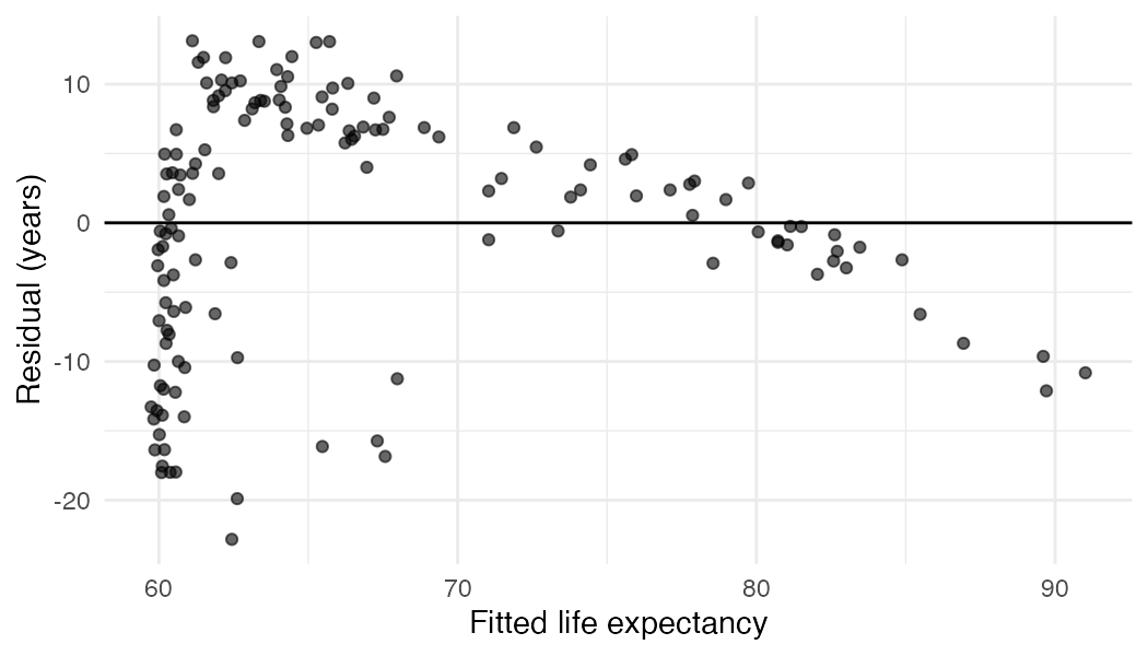
Its residuals: a clear arch, not a cloud. Compare with the residual plot of the log model.

Post your audit

On the Ed thread “AI audit #1”, one post per group:

The problem your group found first, and how
The one you missed, and what would have helped you catch it

Important

The habit: before believing any regression, from an AI, a paper, or yourself: plot the data, plot the residuals, check nobs(), and read every coefficient in its units.

Your project’s first model

For the mid-quarter report

Due Tue, Nov 3: data cleaned by a script, first figures, first model. Start now:

Write the question as “y explained by x”. What’s one row?
Plot y against x. Straight? Does a log help?
fit <- lm(y ~ x, data = ...), then nobs(fit)
One sentence for the slope, in units: “for each …, predicted … is … higher”
The residual plot. Which observations are furthest from the line, and why?

AI is allowed on the report, with disclosure. After today, you know what to check in anything it writes.

Key points

lm(y ~ x, data = df) fits a straight line; coef(), predict(), residuals(), nobs() get its pieces
With log10(x) as predictor, the slope is the change in y per ten-fold increase in x
The intercept is the prediction at x = 0, often outside the data and meaningless alone
R² is the share of variation explained, not accuracy. A small p-value says the slope isn’t zero, not that it matters
Plot the data and the residuals before believing the numbers. Predict only inside the data
Regression describes association, not cause

Before Thursday

DS 5: both PDFs on Canvas by Wednesday 11:59 pm
Ed: your “DS 5 check” post, and your group’s “AI audit #1” post
week05/regression.R restarts and sources cleanly
Project: one plot of your y against your x, and a first lm()

Practice: Lesson 11: Regression in Practice covers everything from today, with your own year of data.

Thursday, Oct 29: Writing Data, Splitting and Combining Data Frames.

AI says	Problem	How you’d find it
“$100,000 → 123 years”	Extrapolation. The data stop at \(49,357 \| `range(gm07\)gdpPercap)`; nobody lives 123 years
“increases”, “should prioritize growth”	Causal claim from observational data	Ask: what else differs between rich and poor countries?
“most important factor”	p-value misread as importance	A p-value is not a size; there’s only one predictor to compare

Linear Regression in Practice

Today’s plan

DS 5 check

Swap laptops

Then, back on your own laptop

Fitting a line

A question worth a line

lm(): a linear model

Read the slope in the units of the data

Predictions

Your turn: two predictions

How good is the line?

summary(): read three numbers

Residuals: what the line misses

The residual plot

Check how many rows the model used

A line is not a cause

AI audit #1

The task

The AI’s analysis

What we found: the numbers

What we found: the conclusions

The plot the AI never made

Post your audit

Your project’s first model

For the mid-quarter report

Key points

Before Thursday

`lm()`: a linear model

`summary()`: read three numbers