Graphics with ggplot2

Week 4 · Thursday, Oct 15 · Lecture

Dr. Marcela Alfaro Córdoba

Today’s plan

Time	What
1:30	Why plot? Data + `aes()` + geom
1:55	Lines, groups and layers
2:15	Mapped vs. fixed; scales and trend lines
2:35	Facets, labels, saving a figure
2:45	Back to the survey: a plot is a check, too
3:00	Tuesday: how the afternoon will run

Learning goals: build a plot layer by layer, decide what is mapped to the data and what is fixed, and say in one sentence why a plot type suits a question.

Laptops open from the start: the DS 3 discussion check moves to Tuesday afternoon, so today is all ggplot2. Still no AI.

Why plot?

Same numbers, four stories

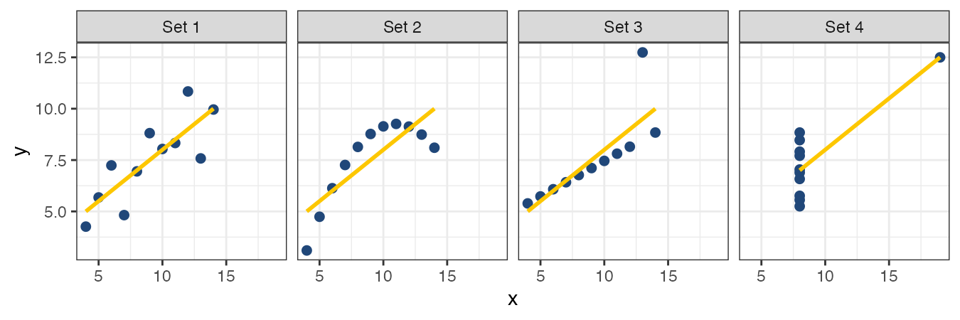
anscombe comes with R. Four small datasets, x1/y1 to x4/y4:

sapply(anscombe, mean)
#>  x1  x2  x3  x4    y1    y2    y3    y4
#>   9   9   9   9  7.50  7.50  7.50  7.50
cor(anscombe$x1, anscombe$y1)    #> [1] 0.816    and 0.816, 0.816, 0.817 for the others

Same means, same SDs, same correlation, same regression line. Only one of them is a straight-line relationship. Look at your data before you summarize it.

Today’s script

Create week04/ggplot2.R:

# Week 4 · Graphics with ggplot2
source("scripts/load-gapminder.R")
source("scripts/check-gapminder.R")

library(ggplot2)

ggplot2 came with the tidyverse you installed in Week 1. library() goes at the top of the script, every time
If you see there is no package called 'ggplot2': install.packages("ggplot2") in the console, never in the script

Tip

Every figure you make today stays in this file. A plot you can’t re-make from a script is a screenshot, not an analysis.

Data + `aes()` + geom

Three parts, joined with `+`

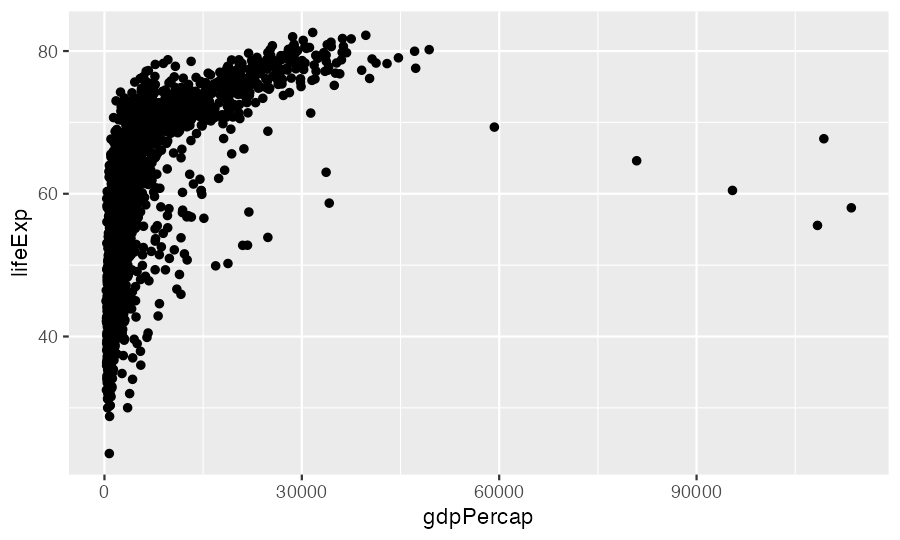
ggplot(data = gapminder, mapping = aes(x = gdpPercap, y = lifeExp)) +
  geom_point()

Part	Says	Here
data	which data frame	`gapminder`
`aes()`	which column goes to which visual property	`gdpPercap` → x, `lifeExp` → y
geom	how to draw each row	a point

This is the grammar of graphics: every ggplot, however fancy, is these three plus optional extras, added with +.

Build it one piece at a time

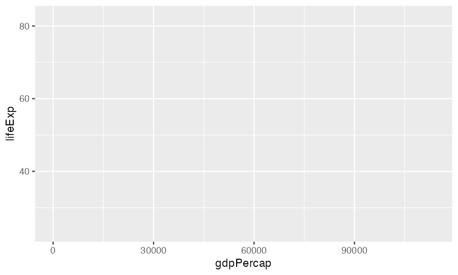
ggplot(gapminder,
       aes(x = gdpPercap, y = lifeExp))

Axes, but nothing drawn: no geom yet.

ggplot(gapminder,
       aes(x = gdpPercap, y = lifeExp)) +
  geom_point()

One point per row: 1704 of them.

The `+` goes at the end of the line

ggplot(gapminder, aes(x = gdpPercap, y = lifeExp))
  + geom_point()
#> Error: Cannot use `+` with a single argument.
#> ℹ Did you accidentally put `+` on a new line?

R ran the first line as a complete command (an empty plot), then hit a line starting with +.

Tip

Same rule as Week 2: R reads a line as finished unless something tells it more is coming. A + at the end of a line says “more is coming”.

Pick the geom from the question

Your question is about…	Geom	Example
a relationship between two numbers	`geom_point()`	GDP vs. life expectancy
change over time	`geom_line()`	life expectancy, 1952-2007
the distribution of one number	`geom_histogram()`	commute times
a number across groups	`geom_boxplot()`	commute by site
counts of a category	`geom_bar()`	survey responses per site

Before you write any ggplot code for your project, write the question in one sentence. The geom usually follows from it.

Your turn: predict, then run

⏱ 5 min

On paper first: what does each one draw? What’s on each axis, and roughly how many marks?

gm07 <- gapminder[gapminder$year == 2007, ]

ggplot(gm07, aes(x = lifeExp)) + geom_histogram(binwidth = 5)

ggplot(gm07, aes(x = continent, y = lifeExp)) + geom_boxplot()

ggplot(gm07, aes(x = continent)) + geom_bar()

Then run them in your script. For each, write one comment with the question it answers.

Distribution of life expectancy in 2007 · how it differs across continents · how many countries per continent (52 Africa, 25 Americas, 33 Asia, 30 Europe, 2 Oceania). geom_bar() needs only x: it counts for you.

Lines, groups and layers

Which points belong to one line?

cr <- gapminder[gapminder$country %in% c("Costa Rica", "Nicaragua", "Panama"), ]
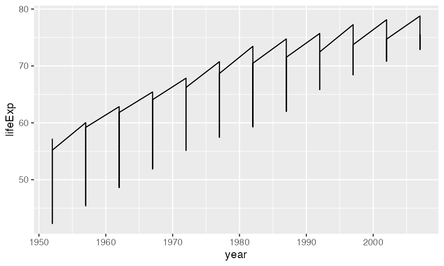
ggplot(cr, aes(x = year, y = lifeExp)) + geom_line()

A saw. geom_line() connected all 36 rows in year order, jumping between the three countries at every year.

`group` says which rows form one line

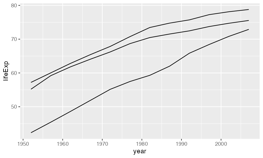
ggplot(cr, aes(x = year, y = lifeExp,
               group = country)) +
  geom_line()

Colour by country and the grouping comes for free:

ggplot(cr, aes(x = year, y = lifeExp,
               colour = country)) +
  geom_line()

A mapped category (colour, shape, linetype) also splits the rows into groups. You need group when nothing else does, as with 142 countries coloured by continent.

Layers draw in the order you add them

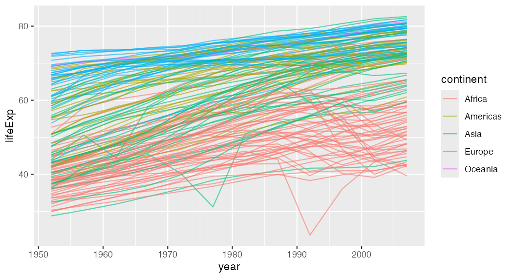
ggplot(gapminder, aes(x = year, y = lifeExp, group = country, colour = continent)) +
  geom_line(alpha = 0.6)

Add + geom_point() and the points sit on top of the lines. Put geom_point() first and the lines cover them. Later layers win.

Mappings are inherited

ggplot(gapminder, aes(x = year, y = lifeExp, group = country)) +   # every layer gets these
  geom_line(aes(colour = continent)) +                            # only the lines get colour
  geom_point()                                                    # points: black

Where you write `aes()`	Applies to
inside `ggplot()`	every layer
inside one `geom_*()`	that layer only

This matters in a minute, when we add trend lines.

Your turn: Andes life expectancy

⏱ 7 min

Last week’s %in%, now with a picture:

Make andes, only the rows for Bolivia, Chile and Peru. Check: 36 rows
Plot life expectancy over time, one line per country, coloured by country
Add points, drawn on top of the lines
Now move colour = country from ggplot() into geom_line() only. What changes, and why?

andes <- gapminder[gapminder$country %in% c("Bolivia", "Chile", "Peru"), ]
ggplot(andes, aes(x = year, y = lifeExp, colour = country)) +
  geom_line() +
  geom_point()

Step 4: the lines keep their colours, the points turn black. The points layer no longer inherits colour.

Mapped vs. fixed

Inside `aes()`: it depends on the data

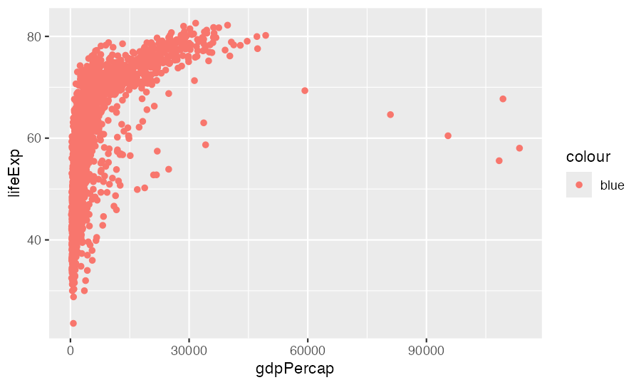
ggplot(gapminder, aes(x = gdpPercap, y = lifeExp)) +
  geom_point(aes(colour = "blue"))

Salmon points, and a legend titled colour with one entry, blue. Inside aes(), "blue" is treated as data: a column whose every value is the word “blue”. ggplot gives that category its first default colour.

Outside `aes()`: the same for every point

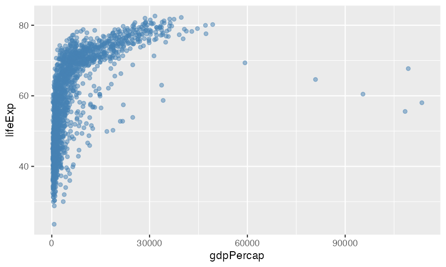
ggplot(gapminder, aes(x = gdpPercap, y = lifeExp)) +
  geom_point(colour = "steelblue", alpha = 0.5)

Property	Example
`colour`	`"steelblue"`, `"#204779"`
`size`	`3`
`alpha`	`0.5` (0 invisible, 1 solid)
`shape`	`17` (filled triangle)
`linewidth`	`1.2` (lines)

alpha is how you see 1704 overlapping points. Shapes are numbered; ?points shows them all.

Depends on a column? Inside aes(). Same for everyone? Outside.

Your turn: fix three plots

⏱ 6 min

Each has one mistake. Fix it, and write the mistake in a comment.

# a) all points orange
ggplot(gm07, aes(x = gdpPercap, y = lifeExp, colour = "orange")) + geom_point()

# b) points coloured by continent
ggplot(gm07, aes(x = gdpPercap, y = lifeExp)) + geom_point(colour = continent)

# c) one line per country, thicker
ggplot(andes, aes(x = year, y = lifeExp, group = country)) + geom_line(aes(linewidth = 2))

colour = "orange" goes in geom_point(), outside aes() · b) continent is a column, so aes(colour = continent). As written: object 'continent' not found, because outside aes() R looks for a variable called continent, not a column · c) a fixed width: geom_line(linewidth = 2). Inside aes(), 2 is treated as data: you get a pointless legend, and the lines aren’t even width 2 (ggplot scales them to 3.5).

Scales and trend lines

A log scale for numbers that span a wide range

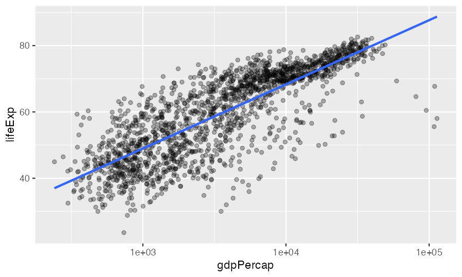
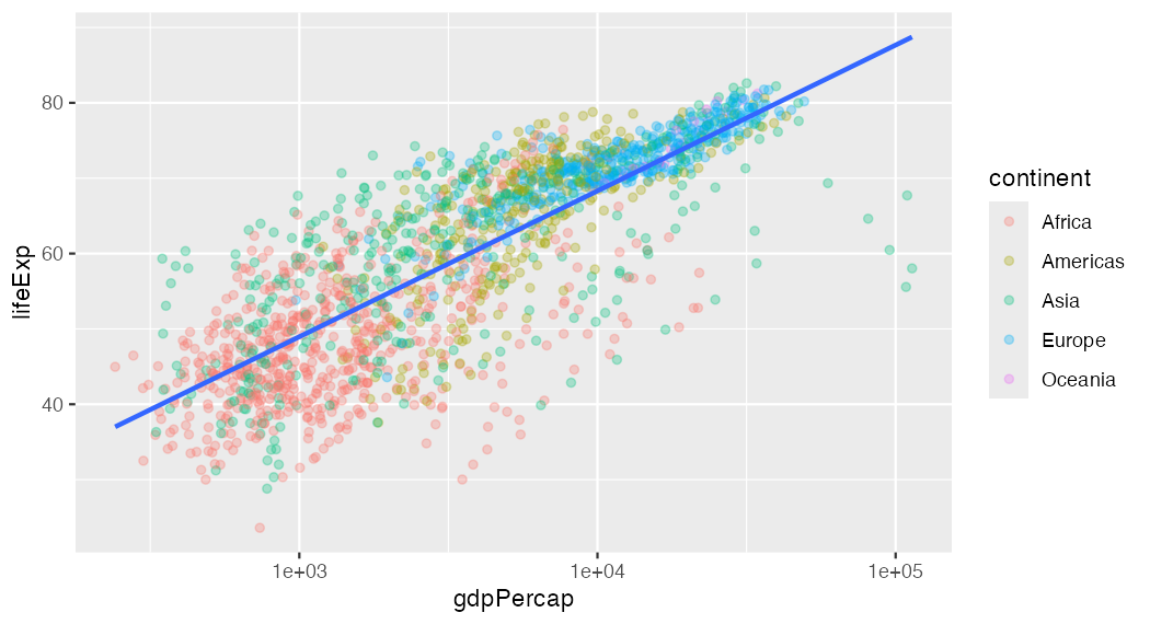
ggplot(gapminder, aes(x = gdpPercap, y = lifeExp)) +
  geom_point(alpha = 0.3) +
  scale_x_log10() +
  geom_smooth(method = "lm", se = FALSE)
#> `geom_smooth()` using formula = 'y ~ x'

GDP runs from about 240 to 113,000. On a log scale each step on the axis is ×10, and the cloud straightens out. The message is information, not an error.

One trend line, or one per group?

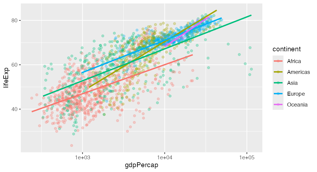
ggplot(gapminder, aes(x = gdpPercap,
    y = lifeExp, colour = continent)) +
  geom_point(alpha = 0.3) +
  scale_x_log10() +
  geom_smooth(method = "lm", se = FALSE)

ggplot(gapminder, aes(x = gdpPercap,
    y = lifeExp)) +
  geom_point(aes(colour = continent),
             alpha = 0.3) +
  scale_x_log10() +
  geom_smooth(method = "lm", se = FALSE)

Left: colour in ggplot(), so geom_smooth() inherits it and fits five lines. Right: colour only on the points, so one line for everyone. Which is right depends on your question.

Facets, labels, saving

Facets: small multiples

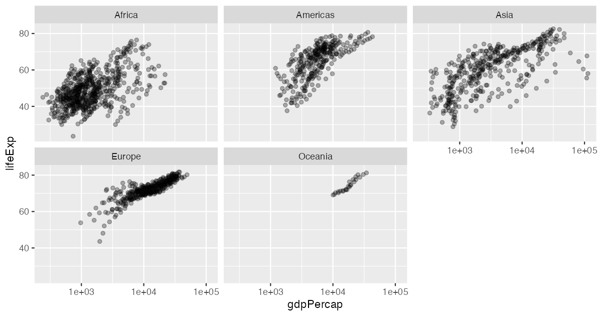
ggplot(gapminder, aes(x = gdpPercap, y = lifeExp)) +
  geom_point(alpha = 0.3) +
  scale_x_log10() +
  facet_wrap(~ continent)

One panel per continent, same axes, so you can compare them. facet_grid(rows ~ cols) does two variables at once. Facets beat five colours when the groups overlap a lot.

Labels a reader can understand

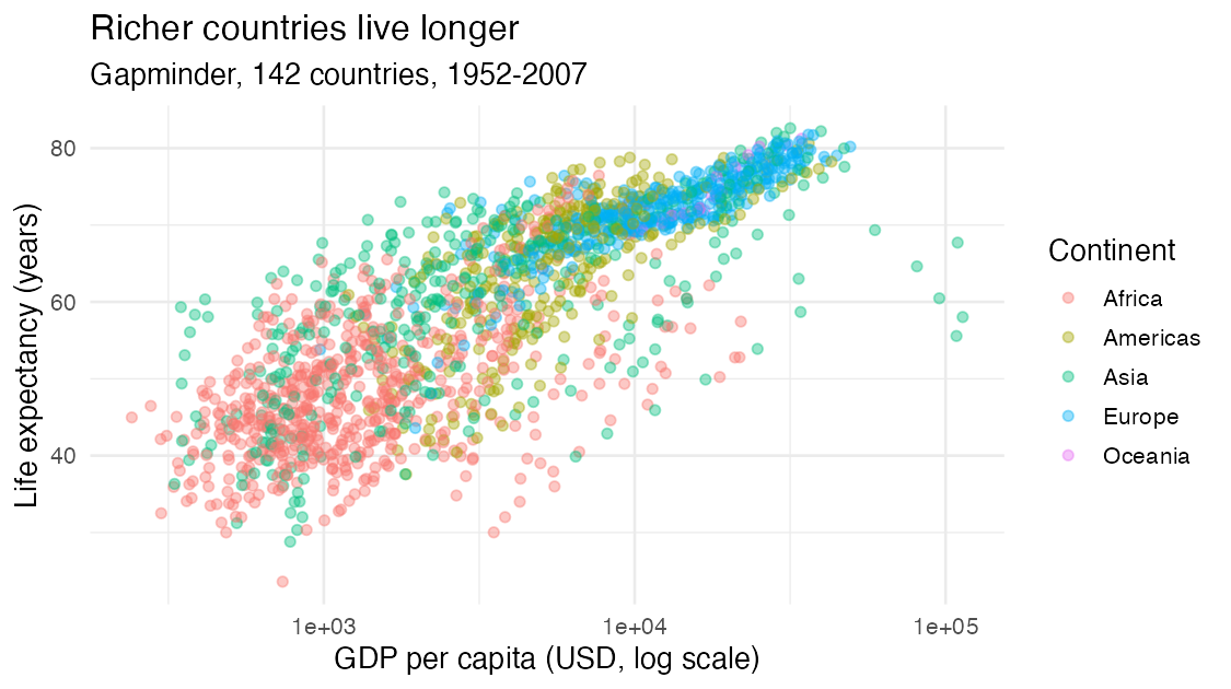
ggplot(gapminder, aes(x = gdpPercap, y = lifeExp, colour = continent)) +
  geom_point(alpha = 0.4) +
  scale_x_log10() +
  labs(x = "GDP per capita (USD, log scale)", y = "Life expectancy (years)",
       colour = "Continent", title = "Richer countries live longer",
       subtitle = "Gapminder, 142 countries, 1952-2007") +
  theme_minimal()

Save it from the script

p_le_gdp <- ggplot(gapminder, aes(x = gdpPercap, y = lifeExp, colour = continent)) +
  geom_point(alpha = 0.4) +
  scale_x_log10() +
  labs(x = "GDP per capita (USD, log scale)", y = "Life expectancy (years)")

p_le_gdp                                       # show it
ggsave("figures/le-gdp.png", p_le_gdp, width = 7, height = 4)

A ggplot is an object: store it, print it, add to it later (p_le_gdp + facet_wrap(~ continent))
ggsave() writes a file. Sizes are in inches; the same code gives the same figure every time
figures/ must exist first: create it once in Positron’s file pane

Important

Never “Export → Save as” from the plot pane for your project. If a reviewer asks you to change the axis label, you want to change one line and re-run, not redo it by hand.

Themes and tweaks

+ theme_minimal()                                   # whole look
+ theme_bw()
+ theme(axis.text.x = element_text(angle = 45))     # one element
+ theme(axis.title.x = element_blank())             # remove one element

theme_*() first, then theme(...) to adjust. The other way round, the full theme resets your tweak. Later layers win, again.

Back to the survey

A plot is a check, too

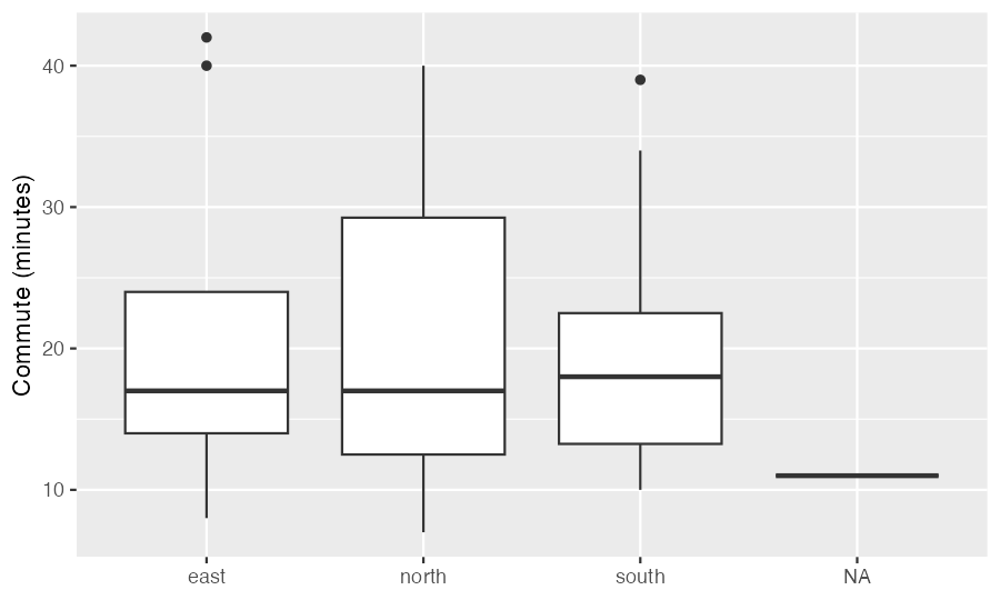
Tuesday’s cleaning script, then one boxplot:

source("scripts/clean-survey.R")
ggplot(survey, aes(x = site, y = commute_min)) + geom_boxplot()
#> Warning message:
#> Removed 1 row containing non-finite outside the scale range (`stat_boxplot()`).

The warning: the 1 row with NA commute (id 35). Expected: colSums(is.na(survey)) said 1
The NA box: the 1 row with no site (id 27). A single value, so a flat line
Neither is a bug. Both are things you should say when you show this plot

Don’t silence warnings you can’t explain

Count the NAs before you plot. Then the warning tells you nothing new.

If the warning says Removed 40 rows and you expected 1, stop. That’s a cleaning bug, not a plotting one.

To drop the NA site from the plot on purpose: ggplot(survey[!is.na(survey$site), ], ...). To keep it, label it (“no site recorded”) and say so in the caption. Either way, it’s a decision you write down.

Your turn: say why

⏱ 8 min

For the survey, write the code and a one-sentence comment saying why this plot type fits:

How long are commutes, overall?
Do people who live farther away visit the library less? (commute_min and visits)
How many responses came from each site?

Then save your favorite with ggsave() into figures/, restart R, and source week04/ggplot2.R to check it re-makes the file.

geom_histogram(): one number, its distribution · 2. geom_point(): relationship between two numbers (try alpha, many share values) · 3. geom_bar(): counts of a category. The sentence is the habit we’re after: you’ll be asked it in every oral component of the project.

Key points

A ggplot is data + aes() + geom, joined with + at the end of each line
Pick the geom from the question: relationship, change, distribution, groups, counts
group says which rows make one line; a mapped category does it too
Later layers draw on top; aes() in ggplot() is inherited by every layer
Inside aes(): depends on the data. Outside: fixed for every mark
scale_x_log10() for wide ranges; geom_smooth(method = "lm") follows the grouping
facet_wrap() for small multiples; labs() for readers; ggsave() from the script
Plot warnings about removed rows should match NA counts you already know

Tuesday, Oct 20

Tuesday is a full day

9:50-10:55 am · DS 4

Lesson 8: Graphics with ggplot2, alone, no AI. Bring the printout to Thursday, Oct 22.

1:30-3:05 pm · DS 3 check + proposals

Bring your DS 3 printout (Lesson 6) and a pencil: the discussion check is first. Then every group presents. Vectorization moves to Thursday, Oct 22.

Proposal: 3 minutes plus questions, each partner answers. Guidelines.

Question · Data (show the first rows, from your load script) · Plan · Risks · Team
AI-use note on your last slide. No AI while presenting or answering
Upload your slides as one PDF to Canvas by 1:00 pm Tuesday, so they’re all on one laptop and we don’t lose time switching

Optional but useful: one exploratory plot of your data, made with today’s code. “Here’s what I already see” is a strong way to explain your plan.

Before you go

week04/ggplot2.R restarts and sources cleanly, and re-makes figures/
library(ggplot2) works on your laptop, so Tuesday’s DS starts on time
DS 3 printout and a pencil packed for Tuesday afternoon
Project: your data loads from scripts/load-<yourdata>.R
Proposal slides: 3 minutes, 5 items, AI note on the last slide

Tonight or tomorrow: read the Lesson 8 page before Tuesday’s DS. The exercises will feel familiar after today.

Next: Tuesday, Oct 20 · DS 4 in the morning, proposals in the afternoon.

Graphics with ggplot2

Today’s plan

Why plot?

Same numbers, four stories

Today’s script

Data + aes() + geom

Three parts, joined with +

Build it one piece at a time

The + goes at the end of the line

Pick the geom from the question

Your turn: predict, then run

Lines, groups and layers

Which points belong to one line?

group says which rows form one line

Layers draw in the order you add them

Mappings are inherited

Your turn: Andes life expectancy

Mapped vs. fixed

Inside aes(): it depends on the data

Outside aes(): the same for every point

Your turn: fix three plots

Scales and trend lines

A log scale for numbers that span a wide range

One trend line, or one per group?

Facets, labels, saving

Facets: small multiples

Labels a reader can understand

Save it from the script

Themes and tweaks

Back to the survey

A plot is a check, too

Don’t silence warnings you can’t explain

Your turn: say why

Key points

Tuesday, Oct 20

Tuesday is a full day

Before you go

Data + `aes()` + geom

Three parts, joined with `+`

The `+` goes at the end of the line

`group` says which rows form one line

Inside `aes()`: it depends on the data

Outside `aes()`: the same for every point